Aug 31, 1994 - Nevertheless, we can recover a methodological insight from the ... recover biological information. A single parameter is ... tree may more easily provide data for a possible biological ...... provided with the floppy disk on request.
J. theor. Biol. (1995) 175, 235–243
A New Method for Evaluating the Shape of Large Phylogenies G F†§ Q C. B. C‡ † Dipartimento di Biologia, Universita` di Padova, via Trieste, 75, I-35121, Padova, Italy and ‡ Royal Botanic Garden, 20A Inverleith Row, Edinburgh EH3 5LR and Institute of Cell Molecular Biology, University of Edinburgh, Kings Buildings, Edinburgh EH9 3JH, U.K. (Received on 31 August 1994, Accepted in revised form on 20 December 1994)
The symmetry of branching of evolutionary trees is considered to be informative of the evolutionary process. Most recent methods for measuring this symmetry (‘‘imbalance’’) measure only one aspect of tree shape. The method we present here provides an almost complete description of tree shape and allows calculation of imbalance parameters for very large phylogenies. The method can detect different patterns of radiation, both among nodes within a tree and among trees. Preliminary tests of the method suggest that bird and angiosperm cladograms have similar tree balance if only the resolved topology of the tree is considered, but very different balance if the dimensions of terminal taxa, measured as number of species, are also included. 7 1995 Academic Press Limited
& Nee, 1993; Harvey et al., 1994a, b) offer an original approach that measures the increase of the number of clades over time in a monophyletic group, comparing and evaluating that behaviour with appropriate null models. A diverse group of studies consider only the topology of phylogenetic trees (see below). The reason for considering what may seem to be a ‘‘reduced information set’’ is that many phylogeny reconstruction methods do not provide branch lengths or, more often, when these are given, there is no guarantee that a reliable molecular clock allows a correct relative timing of branching events. In line with this last group of studies, we offer a novel approach to the study of the topology of large trees, which allows for the incorporation of taxonomic information.
Introduction It is generally believed that the shape of a phylogenetic tree contains clues about the evolutionary process experienced by that group of organisms (Kirkpatrick & Slatkin, 1993; Harvey et al., 1994a). The analysis of macroevolutionary patterns has a strong tradition in palaeontology (e.g. Raup et al., 1973; Gould et al., 1977). However, recent advances in phylogenetic reconstruction make it possible to complement this work using data from extant species (Nee et al., 1992). The last few years have seen the rapid development of techniques to obtain information about pattern in evolution by analysing phylogenetic trees that consider only extant species as the result of the interaction of cladogenesis and extinction. A few studies consider both the topology and the branch length of phylogenetic trees when analysing their structure (Hey, 1992; Brown, 1994). Similarly, Harvey, Nee and co-workers (Nee et al., 1992; Harvey
Within the group of studies that considers only the topological information of phylogenetic trees, several methods have been proposed to evaluate the shape of a phylogeny (Savage, 1983; Shao & Sokal, 1990; Guyer & Slowinski, 1991; Heard, 1992; Kirkpatrick & Slatkin, 1993; Page, 1993; Rogers, 1993, in press;
§ Author to whom correspondence should be addressed. 0022–5193/95/140235+09 $12.00/0
235
7 1995 Academic Press Limited
236
. .
Mooers, in press). The shape is generally understood as a degree of ‘‘symmetry’’ that varies between two extremes: balanced and unbalanced. This symmetry is captured in a single parameter or index. The general aim is to compare the observed symmetry with that expected from null models. Although the more recent methods of analysis (e.g. Kirkpatrick & Slatkin, 1993) are generally well designed and statistically very accurate, most are intended to evaluate the shape of small trees. This may be either because the authors wished to measure the topology of small trees (Guyer & Slowinski, 1991), or because the property of the database required by the method (for instance strictly binary trees, or the need for species as terminal taxa) confines their application to small phylogenies (Heard, 1992; Kirkpatrick & Slatkin, 1993). When supraspecific terminal taxa are considered, or polytomies are allowed (as in Shao & Sokal, 1990), the precision of statistics can be affected (Guyer & Slowinski, 1991; Kirkpatrick & Slatkin, 1993). It is important to realize, however, that if these measures are used with terminal taxa above the species level, they only record the topology of the tree, and do not take into account the differing dimensions (as number of species included) of the terminal taxa. The dubious biological meaning of such measures will be discussed later. Guyer & Slowinski (1993) offer a completely different approach focused on the study of very large phylogenies, in order to recognize the signature of adaptive radiation. Their method evaluates the balance at a single binary node of a large cladogram, measuring the partition of species between the two sister lineages. A major problem with this approach is that a single node does not represent the structure of the whole tree. Also, in order to compare balance and imbalance with a null model, they establish an arbitrary cut-off—either more than 90% of species in one of the two branches (unbalanced) or less than 90% in the bigger branch (balanced)—so symmetry may have only two values without any intermediates. Recently, Sanderson & Donoghue (1994) proposed a statistical method for testing correlation between change in diversification rate during the evolution of a group and the evolution of presumed key characters. They studied the evolutionary radiation of angiosperms by evaluating disparity in species diversity among clades in three-taxon phylogenies. This method aims to identify the causes of evolutionary radiation in individual study cases and does not deal with the recurrence and the magnitude of radiation in evolutionary history.
Similar problems have been addressed in the past through analysis of biological classifications (Willis, 1922; Cronk, 1989; Dial & Marzluff, 1989; Burlando, 1990, 1993; Minelli et al., 1991). These approaches concentrate on the geometry of biological diversity more than on the reconstruction of a historical process (Minelli et al., 1991). The classification approach is supported by larger databases and produces clear patterns in the form of frequency distributions. However, because it deals with classifications and not trees, it is not well suited to the study of evolutionary history. Nevertheless, we can recover a methodological insight from the classification approach: the use of frequency distributions as a means of looking at the geometry of nature, and the use of classifications to recover biological information. A single parameter is unlikely to be sufficient to describe in a biologically meaningful way the topology of a phylogeny, especially if this is quite large. An analysis that offers a more comprehensive view of the tree may more easily provide data for a possible biological explanation. A More Complete View of Tree Symmetry Our method aims to combine information from phylogeny and classification in order to discover clues to evolutionary patterns of speciation and extinction in the shape of a phylogenetic tree. It is primarily designed for the study of large trees, but small tree analysis is also feasible. It may be considered a development of Guyer & Slowinski’s (1993) method: here the analysis of balance is extended to the whole tree while maintaining the claim that only sister group comparisons are informative. In this vein, we regard as informative not only the topology of the branching but also the full weight of unresolved cladogenesis within the terminal nodes. We think that this perspective of symmetry may allow better correlation with other biological information. The features that make our approach particularly suited to the study of large phylogenies are: , terminal taxa may be species as well as groups above the species level, up to any rank; , a certain proportion of polytomies are allowed; , to a certain extent, incomplete phylogenies can be analysed; , the output in two steps gives first a comprehensive view of the shape as a frequency diagram and then provides a measure of symmetry via descriptive statistics.
In order to simplify the following discussion we introduce two definitions: the size of a node is the number of species that it subtends; the imbalance of a node (defined only for binary internal nodes) is the degree of symmetry in the partition of species between the two sister clades that originate from that node. We shall describe the shape of a phylogenetic tree as the frequency distribution of the imbalance of its nodes. Our analysis may be easily explained as a four-step procedure. 1. Building the data set In the most general case, building the data set needs three kinds of biological information. These may come from the same source but in general it will be necessary to combine different sources of data, as follows: (i) A branching diagram (cladogram or phenogram). Terminal taxa are not necessarily species and also a few polytomies are allowed. Branch length is not considered. (ii) The dimension (as number of species) of each terminal taxon. (iii) An assessment of whether the terminal taxa constitute reasonably uniform taxonomic groups. Indeed, because of the incomplete resolution of the tree (terminal taxa may be considered as terminal polytomies), the nodes we consider are only a sample of the statistical universe of nodes of that phylogeny. The sample needs a useful biological meaning (O’Hara, 1992; Sillen-Tullberg, 1993). We consider evolutionarily reasonable the set of nodes that represent the cladogenetic events that occurred before a certain moment in geological time. If some terminal taxa are older than that date we will miss some meaningful items of node imbalance hidden in their grouping. If some taxa are younger, we will take into account, for a certain part of the tree, more nodes than in the remainder of the tree, thus biasing the sample. If a good fossil record or a reliable molecular clock are available, it is possible to reduce the mis-sampling of the nodes of the tree. Combining all this information, we obtain a tree that can be represented as a Venn diagram in which brackets give the topology of the phylogeny and figures within the brackets give the dimensions of the terminal taxa. Moreover, the whole data set can be easily split into sub-units in order to analyse different parts of the same tree.
237
Each internal binary node of the resultant tree represents a clade divided into two sister groups. It is possible to associate each of these nodes with a value of imbalance that represents the partition of species between the two sister branches. 2. Calculation of the node imbalance Of the several ways to calculate the degree of unequal partition of species between the two lineages that originate from a node, we use the following measure that accounts for the dimension of the bigger branch in relation to its maximum possible size. The mathematical meaning is clear, the range of possible values is finite and independent of the size of the node. Let S represent the size of the node and B the size of the bigger branch (S must be larger than 3, as 2- and 3-species binary sub-trees lack alternative topologies). For a node of size S, the minimum dimension for the bigger branch (B) is: m=(S div 2)+(S mod 2), where div is the integer division operator and mod gives the remainder of an integer division (if S is an even number, this expression is equivalent to m=S/2). The maximum size for the bigger branch (B) is: M=S−1, so the range of possible values for the bigger branch is the closed interval [m, M]. For instance, for S=21, m=10+1=11 and M=20. We define the imbalance of the node (I ) as the ratio between the observed deviation of the bigger branch from the minimum value of its range and the amplitude of that range, that is: I=(B−m)/(M−m). I takes values from 0 to 1 inclusive. I=0 if the bigger branch has the minimum dimension (B=m), i.e. the node has maximum balance. I=1 when B=M, thus having the maximum imbalance, i.e. when all the species but one belong to a single lineage. For example, a node with ten species (S=10), partitioned as 3:7, has a value of I=(7−5)/(9−5)=0.5. Although the parameter I may assume only a finite number of values in the interval [0, 1], because B can only assume discrete values, the magnitude of I is independent of S, allowing the study of the frequency distribution of I in a tree with nodes of different sizes (see below).
. .
238 3. Frequency distribution diagrams
In a N-tipped binary tree there are N−1 internal nodes (including the root). So there are N−1 pairs of sister clades that may be compared on the basis of their relative dimension. If one of the two taxa is far larger than the other, the node is considered as very unbalanced. On the other hand, if the two taxa are roughly the same size, the node is regarded as balanced. Nodes with less than four species are not considered because the topology of the following sub-tree is constrained to simple and uninformative two- or three-taxa statements. Nodes with more than two daughter branches are also excluded from the analysis: it is impossible to perform a comparison between sister taxa so they are treated as missing data. As this method has been designed mainly to consider large phyloge-
nies, polytomies are not charged with any biological meaning but rather regarded as cases of unresolved relationship (soft polytomies). We reject the option of averaging the imbalance of all the possible dichotomous resolutions of a polytomy. This is because when the order of the polytomy (number of branches attached at the same node) is increased, the ratio of right to wrong solutions quickly decreases, thus risking the inclusion of more noise than information. For this reason we simply exclude polytomies from the set of informative nodes. Polytomies lower the number of possible comparisons, and for this reason their number must be relatively low and they must not be concentrated in a particular region of the tree if we are to have reliable results. We represent the frequency distribution of the imbalance of the nodes as a histogram with ten classes of equal range (Fig. 1).
F. 1. Frequency distribution of the imbalance of the nodes in four phylogenies.
We have already noted that because the number of species can assume only discrete values, for a node of a certain size (S), I may assume only a finite number of values between 0 and 1 (i.e. S div 2). Grouping the measures of node imbalance in classes allows the conversion from a discrete to a continuous distribution in the interval [0, 1]. However, despite the grouping, even in a perfectly equiprobable tree with all possible topologies occurring with equal frequency for each node size, the distribution would not be perfectly uniform. It is easy to eliminate this distortion with an algebraic correction (see Appendix A). From a statistical point of view, this correction is necessary only for small trees with a good percentage of small terminal taxa (number of species per terminal taxon Q10). For larger trees, because of the large range of node size, these effects are small and tend to cancel each other out, so that the observed frequency distribution is statistically indistinguishable from the corrected one. Nevertheless, for precision and for uniformity of treatment we will apply corrections to all the trees we consider. Different observed distributions can be directly compared with each other or against the distribution of appropriate null models, using non-parametric tests. Alternatively, they can be fitted with a statistical distribution on the basis of the geometry of observed frequency distribution or on the basis of an appropriate biological hypothesis. Frequency distributions offer a first comprehensive view of the way in which the imbalances have been iterated in the evolution of the study group. However, summary statistics can also be taken from the frequency distributions. It is possible to use both the parameter of fitting (if curves have been fitted) or descriptive statistics. 4. Descriptive statistics As our sample of trees is small, we decided to use only the simplest statistical descriptors of shape for the observed distributions. Further work with more data will allow optimal, and more complex, statistics to be assessed. Because of the general asymmetry of observed frequency distributions, we chose the median as the measure of location (central tendency) and the quartile deviation (half the difference between third and first quartile) as the statistic of dispersion. Without involving any biological hypothesis, these parameters describe well the shape of the distribution and allow a statistical comparison with a null model. The median represents the general imbalance of the tree and the quartile deviation expresses the way in which variation in asymmetry of branching have been iterated with respect to the global imbalance.
239
The program for calculating the node imbalance frequency distribution and related statistics is available from the first author on request (see Appendix B). The null model used in this analysis is the so-called Markov model (technically an equiprobable Markov model but we do not use this term to avoid possible confusion with other non-Markovian equiprobable null models of tree shape [cf. Simberloff et al., 1981]). Its main assumption is that the phylogeny is the product of random branching. This results when the ‘‘effective speciation rate’’ (the difference between extinction and speciation rate) is equal for all species. The effective speciation rate may change through time, provided that it is the same for all lineages at a given time. Because of its simple assumptions, it is generally considered the most suitable null model for bifurcating phylogeny in biology (Heard, 1992; Rogers, in press). It is easy to demonstrate that the frequency distribution of the imbalance of the nodes for a Markovian tree converges quickly to a uniform distribution in the interval [0, 1] as the size of the tree increases. This is because in a Markovian tree, for a node of any size, all the possible partitions of species between the two lineages are equally probable (for a formal demonstration, see Farris, 1976). In order to compare the shape of imbalance distribution between the null model and observed trees, we studied the distribution of the median and quartile deviation in Markovian trees. The median and the quartile distribution for a uniform distribution in the interval [0, 1] are 0.5 and 0.25, respectively. Because of the non-normal character of node imbalance distribution, we studied the distribution of the two sample statistics by computer simulation. The width of the confidence interval for the two statistics depends on the dimension of the tree: both the number of terminal taxa and their global size. The simulation constructs a random tree of a given size (number of species and informative nodes as in the observed tree) and then calculates the two statistics. This procedure is repeated enough time to estimate the 95% confidence intervals. Preliminary Test of the Method Three phylogenies (two large and one smaller) were chosen to test this new approach. In a recent paper, Chase et al. (1993) presented two large consensus cladograms for seed plants, based on DNA sequence analysis of the rbcL gene. The species
240
. .
studied represent all major taxonomic groups. On the basis of these two cladograms we constructed two different trees for angiosperms that have families as terminal taxa. The two original cladograms differ in the number of species analysed (475 and 499 respectively) and in the consensus criteria adopted. In the following discussion we refer to them as tree a for the smaller one) and tree b, according to the labels adopted in the published cladograms. Numbers of species in each family were taken from Mabberley (1993). Where the classification adopted in Mabberley could not be used because the families are para- or polyphyletic with respect to the cladogram, we used a list of genera per family (Brummitt, 1992) to estimate the number of species in each terminal clade. In the rare cases where neither approach could solve the problems with the topology of the cladogram, those paraphyletic families were included only at the level of lower unproblematic nodes. Polyphyly involving two or three families was solved by grouping those families in a single clade. In cases of very widespread polyphyly, to avoid lumping too many terminal taxa (thereby losing information) we decided to consider the new terminal clades as families. Their sizes were estimated by considering the size and affinities of the genera that represented them in the cladogram. Finally, we lumped a few terminal taxa (reducing the total of about 10%) on the basis of the fossil survey of Collinson et al. (1993) and Eriksson & Bremer (1992), in order to improve the uniformity of the taxonomic units. Because of weaknesses in the plant fossil record (Collinson et al., 1993), we adopted a slight correction, lumping the nodes supposed younger than 20 million years. The main problem with this tree is that not all the families of living plants have been included in the analysis. About 100 out of some 400 families recognized by Mabberley (a total of 10000 species) are excluded from our calculation. As most of the missing families are small or very small taxa, we can predict the likely effect of this bias. It is reasonable to expect that, generally, their inclusion in the tree would not affect the imbalance of included nodes because of the large size of the latter. However, unless all the small taxa are closely related, their inclusion might produce new unbalanced nodes. The global imbalance (median) of this phylogeny may therefore be underestimated. As is discussed below, the more complete angiosperm tree has a higher median, so apparently confirming this interpretation. The general resemblance of these frequency distributions to those of complete phylogenies may also indicate the lack of any strong bias. From this large phylogeny we obtained another four large sub-trees for some monophyletic groups:
eudicots, non-eudicots, rosids and asterids (for details, see Chase et al., 1993). We analysed Sibley & Ahlquist’s (1990) UPGMA phenogram of birds derived from DNA–DNA hybridisation studies. The phenogram is based on data from a sample of some 1700 of the c. 9700 species of living birds. We restricted our analysis to consider Sibley and Ahlquist’s families as terminal taxa. In this way all extant lineages are included in the calculation of balance. The dimension of the terminal taxa follows Sibley & Monroe’s (1990) world catalogue. In the dendrogram, branching events are assumed to have a relative chronology, so we avoid having to include any correction for non-uniformity of terminal taxonomic units. From this phylogeny we analysed three trees of the largest groups: all birds, and two monophyletic subgroups, Passeriformes and Ciconiiformes. Anthemideae is one of the larger tribes in the plant family Asteraceae (Compositae). Bremer & Humphries (1993) provided a cladogram based on morphological characters for all the genera as well as the number of species belonging to each genus. Because these are considered to be reasonably uniform taxonomic units, no correction for unequal resolution has been applied. From this phylogeny we obtained a single tree of the whole tribe. Results and Discussion In all the observed trees, the frequency distributions of the dimension of the nodes are quite skewed (see for example trees in Fig. 1). This results in a median value that is statistically significantly larger than that expected from the null model (Fig. 2). Although the shapes of the frequency distributions look variable, in the main they show an underlying regularity of structure. We do not propose to discuss this regularity further because of the small size of our sample and because the possible biological meaning, if any, is not clear. Observed trees show a more unbalanced structure than Markovian trees. Our result confirms for large phylogenies what analyses of smaller ones had already suggested (Guyer & Slowinski, 1991; Heard, 1992; Mooers, in press). This result also holds true if we apply our method just to the topological structure of the tree (i.e. not considering the different dimensions of the taxa, but instead making all dimensions of terminal taxa equal to one). This procedure, in effect, assumes the same concept of symmetry adopted by
241
F. 2. Bivariate scattergram for the 14 trees analysed, with respect to median and quartile deviation of the frequency distribution of the imbalance of the nodes. Letters refer to the following trees (in brackets the number of informative nodes and species): Aa, angiosperm cladogram a (194, 213250); Ea, eudicots a (127, 154528); Ra, rosids a (59, 63636); Sa, asterids a (57, 85960); Na, non-eudicots a (65, 58720); Ab, angiosperm cladogram b (191, 229660); Eb, eudicots b (138, 169806); Rb, rosids b (67, 68143); Sb, asterids b (49, 86225); Nb, non-eudicots b (51, 59852); T, Asteraceae, Anthemideae (61, 1741); B, birds (133, 9653); P, Passeriformes (41, 5699); C, Ciconiiformes (28, 1027). See text for taxonomic details. In the upper left corner (0.5, 0.25) is the Markovian tree. The 95% confidence intervals for two different tree sizes (the number of nodes and species are given in brackets) are shown as dashed lines.
previous works (by analysing terminal taxa treated as single species), and so makes our method exactly comparable to, for instance, Heard’s (1992) method. Although we cannot see in this measure a special biological meaning, separating the different contributions of tree topology and taxonomic information to the tree symmetry may allow the study of possible biases in phylogenetic reconstruction methods. With this sort of analysis (topology only) the median and quartile deviation of birds are 0.75 and 0.23 respectively; for angiosperms b, the two statistics are 0.74 and 0.24. This is a remarkable agreement in tree balance between two groups that differ greatly in method of analysis (cladogram vs. phenogram) and organism type (plants vs. birds). However, when the full analysis is performed, taking into account the dimension of the terminal taxa, a marked difference emerges. This implies that taking the full weight of phylogeny in the terminal taxa is highly significant in estimating tree balance. Thus, it is a useful feature of the present method that it can include or exclude the terminal polytomies so easily. There appears to be a consistent difference in the median of angiosperms a and angiosperms b. Angiosperms b is a more complete sample of families and has the higher median, supporting the idea we have discussed above that the sampling of families has been non-random with respect to size. A complete tree of angiosperm families might be even more unbalanced, so contrasting with the complete tree of Anthemideae
genera (T) which has a median intermediate between birds and angiosperm families. These intriguing results point to a combination of evolutionary signal and bias of tree-building methodology in producing the observed imbalance. The frequency distribution diagram can reveal differences in tree shape that single statistical parameters cannot recover (see, for instance, the different frequencies of the most balanced nodes of rosid and asterid clades in Fig. 1). Our method detects the nodes that are involved in a pattern of particular interest, allowing a better correlation with any biological process that might have produced those patterns. Our measure of node imbalance could be used with approaches different from the study we present here. For instance, although there is no relative chronological information in a tree if just the topology is considered, actually ordered sequences of cladogenetic event are recorded along the individual lineages. The cladogenetic event represented by the bifurcation of a node must precede in time the cladogenetic events in each of the two daughter branches. We looked for possible correlation between the imbalance of father and daughter nodes in birds phylogenetic tree, and found none. In other words, there is no evidence of ‘‘heritability of node imbalance’’. This approach deserves a more detailed analysis, and we shall consider it in a future paper. From a practical view point, our method is intuitive and produces easily understood geometrical
. .
242
parameters. However, we regard the main advantage of our approach to be the fact that each node is laden with the weight of complete evolutionary history. The pattern of iterative radiation can be related to the pattern of occurrences of character-state transitions that are supposed to be ‘‘key innovations’’ in the evolution of the group. We suggest that our measure reflects the biological phenomenon of radiation more closely than any simple parameter that describes only the topology of branching. Our small sample cannot guarantee that the observed pattern is caused by evolutionary history. If the phylogenies we analysed are inadequate representations of evolutionary history (either because of lack of knowledge or the occurrence of systematic bias in the phylogenetic reconstruction techniques), our results may be of little biological relevance. However, modern molecular phylogenetic methods are improving, phylogenetic information is growing very fast, and many more trees will soon be available for topological analysis (Harvey & Nee 1993; Sanderson et al., 1993: Hillis et al., 1994). Radiation is a central concept in evolutionary biology, expressed in evolutionary trees by nodal imbalance, which is an apparently general pattern of tree shape. Methods that measure the imbalance of trees and individual nodes can be expected to be of central importance in the study of the history of life. If radiation can be identified and explained, we will have achieved a high level of knowledge of the evolutionary process. The method proposed here can be used both to compare trees and to correlate them with different features of an organism, and also can be used to analyse on a node-by-node basis correlation with character-states along the branches of the tree.
We thank A. � O. Mooers and A. Minelli for helpful advice and useful comments at several stages of this study, and D. Foddai and R. Bateman who read an earlier version of the manuscript. The work has been partly supported by a grant from the Erasmus Network in Systematic Biology and a grant from the Italian C.N.R. (research line ‘‘Adaptation and cladogenesis’’ within the project ‘‘Integrated biological systems’’ at the Department of Biology, Padova).
REFERENCES B, K. & H, C. J. (1993). Generic monograph of the Astreraceae-Anthemideae. Bull. nat. Hist. Mus. Lond. (Bot.) 23, 71–177. B, J. K. M. (1994). Probabilities of evolutionary trees. Syst. Biol. 43, 78–91. B, R. K. (1992) Vascular plant families and genera. Whitstable, Kent: Whitstable Litho Ltd. B, B. (1990). The fractal dimension of taxonomic systems. J. theor. Biol. 146, 99–114.
B, B. (1993). The fractal geometry of evolution. J. theor. Biol. 163, 161–172. C, M. W., S, D. E., O, R. G., M, D., L, D. H., M, B. D., D, M. R., P, R. A., H, H. G., Q, Y.-L., K, K. A., R, J. H., C, E., P, J. D., M, J. R., S, K. J., M, H. J., K, W. J., K, K. G., C, W. D., H´, M., G, B. S., J, R. K., K, K.-J., W, C. F., S, J. F., F, G. R., S, S. H., X, Q.-Y., P, G. M., S, P. S., S, S. M., W, S. E., G, P. A., Q, C. J., E, L. E., G, E., L, G. H. J., G, S. W., B, S. C. H., D, S. & A, V. A. (1993). Phylogenetics of seed plants: an analysis of nucleotide sequences from the plastic gene rbcL. Ann. Missouri Bot. Gard. 80, 528–580. C, M. E., B, M. C. & H, P. L. (1993). Magnoliophyta (‘Angiospermae’). In: The Fossil Record 2 (Benton, M. J., ed.) pp. 809–841. London: Chapman & Hall. C, Q. C. B. (1989). Measurement of biological and historical influences in plant classifications. Taxon 38, 357–370. D, K. P. & M, J. M. (1989). Nonrandom diversification within taxonomic assemblages. Syst. Zool. 38, 26–37. E, O. & B, B. (1992). Pollination systems, dispersal modes, life forms, and diversification rates in Angiosperm families. Evolution 46, 258–266. F, J. S. (1976). Expected asymmetry of phylogenetic trees. Syst. Zool. 25, 196–198. G, S. J., R, D. M., S, J. J., S, T. J. M. & S, D. S. (1977). The shape of evolution: a comparison of real and random clades. Paleobiology 3, 23–40. G, C. & S, J. B. (1991). Comparison of observed phylogenetic topologies with null expectations among three monophyletic lineages. Evolution 45, 340–350. G, C. & S, J. B. (1993). Adaptive radiation and the topology of large phylogenies. Evolution 47, 253–263. H, P. H., H, E. C., M, A. � O. & N, S. (1994a). Inferring evolutionary process from molecular phylogenies. In: Models in Phylogenetic Reconstruction (Scotland, R. W., Siebert, D. J. & Williams, O. M., eds) pp. 319–333. Systematic Association Special Volume Series. N. 52. Oxford: Clarendon Press. H, P. H., M, R. M. & N, S. (1994b). Phylogenies without fossils. Evolution 48, 523–529. H, P. H. & N, S. (1993). New uses for new phylogenies. Eur. Rev. 1, 11–19. H, S. B. (1992). Patterns in tree balance among cladistic, phenetic, and randomly generated phylogenetic trees. Evolution 46, 1818–1826. H, J. (1992). Using phylogenetic trees to study speciation and extinction. Evolution 46, 627–640. H, D. M., H, J. P. & C, C. W. (1994). Application and accuracy of molecular phylogenies. Science 264, 671–677. K, M. & S, M. (1993). Searching for evolutionary patterns in the shape of phylogenetic tree. Evolution 47, 1171–1181. M, D. J. (1993). The Plant Book. Cambridge: Cambridge University Press. M, A., F, G. & S, S. (1991). Self-similarity in biological classifications. BioSystems 26, 89–97. M, A. � O. (in press). Tree balance and tree completeness. Evolution. N, S., M, A. � O. & H, P. H. (1992). Tempo and mode of evolution revealed from molecular phylogenies. Proc. natn. Acad. Sci. U.S.A. 89, 8322–8326. O’H, R. J. (1992). Telling the tree: narrative representation and the study of evolutionary history. Biol. Phil. 7, 135–160. P, R. D. M. (1993). On describing the shape of rooted and unrooted trees. Cladistics 9, 93–99. R, D. M., G, S. J., S, T. J. M. & S, D. S. (1973). Stochastic models of phylogeny and the evolution of diversity. J. Geol. 81, 525–542. R, J. S. (1993). Responses of Colless’ tree imbalance to number of terminal taxa. Syst. Biol. 42, 102–105.
R, J. S. (in press). Central moment and probability distribution of Colless’ coefficient of tree imbalance. Evolution. S, M. J., B, B. G., B, G., C, C. S., V D, C., F, D., P, J. M., W, M. F. & D, M. J. (1993). The growth of phylogenetic information and the need for a phylogenetic data base. Syst. Biol. 42, 562–568. S, M. J. & D, M. J. (1994). Shifts in diversification rate with the origin of angiosperms. Science 264, 1590–1593. S, H. M. (1983). The shape of evolution: systematic tree topology. Biol. J. Linn. Soc. 20, 225–244. S, K. & S, R. R. (1990). Tree balance. Syst. Zool. 39, 266–276. S, C. G. & A, J. F. (1990). Phylogeny and Classification of Birds. New Haven: Yale University Press. S, C. G. & M, B. L. J. (1990). Distribution and Taxonomy of Birds of the World. New Haven: Yale University Press. S-T, B. (1993). The effect of biased inclusion of taxa on the correlation between discrete characters in phylogenetic trees. Evolution 47, 1182–1191. S, D., H, K. L., MC, E. D. & C, E. F. (1981). There have been no statistical tests of cladistic biogeographical hypotheses. In: Vicariance Biogeography: A Critique (Nelson, G. & Rosen, D. E., eds) pp. 40–63. New York: Columbia University Press. W, J. C. (1922). Age and Area. Cambridge: Cambridge University Press.
243
distribution simply on the basis of the size frequency of its nodes and the number of classes of the final diagram. These values are algebraically combined with observed values to allow the construction of a frequency distribution with nodes of different size. This is trivially expressed as the formula: Fi=Oi−Ci where Fi is the corrected frequency of the ith class, Oi the observed frequency of the ith class, and Ci the deviation of the expected equiprobable value from the value of a uniform distribution (i.e. 0.1, for a ten-class histogram) for the same class. For large phylogenies, the effect of these biases is insignificant and the observed and corrected frequency distributions are practically indistinguishable.
APPENDIX B The Program Input
APPENDIX A Correction Consider a tree with 100 nodes of size 8. There are four different possible partitions of species within an eight-species clade: 4:4, 5:3, 6:2 and 7:1. The respective imbalance scores for the four partitions are: 0, 0.33, 0.66, 1. Suppose there are exactly 25 nodes for each type, that is to say that each degree of imbalance has the same frequencies of occurrence in the tree. If we plot this distribution as a histogram where I interval [0, 1] is divided into ten classes numbered from 0 to 9, the frequency distribution of balance will be quite different from a uniform distribution simply because there are no topologies that can score in the classes, 1, 2, 4, 5, 7, 8. So the expected equal distribution for a set of nodes with size 8 is: 0.25, 0, 0, 0.25, 0, 0, 0.25, 0, 0, 0.25—quite different from a uniform distribution. As the dimension of the nodes increases, the frequency distribution of the equiprobable node imbalance tends to converge to a uniform distribution. For a 128-species node, rounding at the second decimal digit, values are: 0.11, 0.09, 0.09, 0.11, 0.09, 0.09, 0.11, 0.09, 0.09, 0.11. For a given tree, it is possible to calculate deviation of the equiprobable distribution from the uniform
—Name of a text file that lists one or more trees. Each tree must have a label (name) and will be represented as a Venn diagram where brackets give the topology of the phylogeny and figures give the dimension of the terminal taxa. —Name (label) of the tree to be analysed. —Kind of analysis: considering or not considering the dimension of terminal taxa. Output —Table with, for each binary node, size, dimension of the two lineages and imbalance value (useful to check that the arrangement of the brackets is correct!). —Table of the frequency distribution of observed values, the correction applied, and the corrected data. —Graph of frequency distribution of corrected data with median (M) and quartile deviation (QD). —95% confidence intervals for M and QD for a Markovian tree of the same size calculated by computer simulation. The program, written in Borland Turbo Pascal, a brief description of the algorithm and some examples will be provided with the floppy disk on request.