taneous emission model PHEM (Passenger car and Heavy-duty. Emission ... used to estimate vehicle emissions and fuel consumption. ..... data storage of the trajectory data and computation time of PHEM should be improved if the tool will be. 37 ... CD-ROM of 80th Annual Meeting, Transport Research Board, Wash- ington ...
2010 13th International IEEE Annual Conference on Intelligent Transportation Systems Madeira Island, Portugal, September 19-22, 2010
MA2.2
A New Method to Calculate Emissions with Simulated Traffic Conditions Karin Hirschmann, Michael Zallinger, Martin Fellendorf, Stefan Hausberger Abstract— Microscopic traffic simulation models coupled with instantaneous emission models have the potential to provide improved assessments of the environmental impact of traffic networks, management strategies and technology implementations. This paper describes a toolbox, which links the microscopic traffic flow simulator VISSIM with the instantaneous emission model PHEM (Passenger car and Heavy-duty Emission Model). PHEM was developed to simulate a full fleet of heavy-duty vehicles, passenger cars and light commercial vehicles. The supporting data-set includes gasoline and diesel vehicles from EURO 0 to EURO 6. PHEM calculates vehicle fuel consumption and emissions, using speed trajectories as model input. VISSIM is able to supply these necessary speed profiles for all vehicles within the network. In order to supplement realistic traffic volume with traffic control strategies an interface between VISSIM and the adaptive Urban Traffic Control System MOTION by Siemens has been developed. This paper discusses the evaluation of the modeled traffic situations in urban road network with VISSIM and PHEM by measurements on the road and on the chassis dynamometer. Intensive calibration of the traffic flow simulation has been conducted to match the vehicles’ ’acceleration’ and ’desiredspeed’ parameters to the local conditions. Comparative driving cycles, from the ’on-road’ measurements recorded via GPS instrumented vehicles and the ’virtual’ network simulations were selected. The ’on-road’ and ’virtual network’ driving cycles were measured on the chassis dynamometer with a EURO 4 diesel car. The measurements were compared with the PHEM predictions. This approach allowed the uncertainties associated with modeling speed profiles to be compared with the uncertainties related to the emission model. The overall model performance was evaluated by comparing the PHEM emission calculations based on simulated speed profiles with the measured emissions from the ’on-road’ driving cycles.
I. INTRODUCTION Statistical methods as well as physical models are being used to estimate vehicle emissions and fuel consumption. The variety of models is given by the variety of applications which greatly differ in terms of study purpose. When modeling traffic flow and traffic induced emissions three levels of detail exist: • Microscopic traffic flow simulation and instantaneous emission models • Traffic network and emission models (mesoscopic) • Inventory models (macroscopic) Macro- and mesoscopic emission models like COPERT or HBEFA are used for general considerations like national emission inventories or large road networks where the analysis of single vehicles is usually not required. Microscopic traffic flow simulation models are becoming 978-1-4244-7658-9/10/$26.00 ©2010 IEEE
increasingly popular tools to analyze traffic operations and evaluate traffic management strategies. They simulate single vehicle movements stochastically within welldefined road networks. They are able to simulate complex traffic situations; thus network impacts of different signal control and Intelligent Transport Systems strategies are being evaluated. As microscopic traffic simulation models simulate the time-space trajectories of all vehicles through a network, disaggregate information can be collected and supplied to instantaneous emission models. In the majority of studies up to now, the range of pollutants, and the characterization of the vehicle fleet composition is limited. The emission model PHEM (Passenger car and Heavy Emission Model [3]) is based on engine emission maps. It considers effects of transient load changes. There is a high potential of applications, if a microscopic traffic simulator and an instantaneous emission model is coupled. Detailed modeling on both sides allows evaluating the environmental effect of road network conditions, traffic management strategies, and different signal timings. Furthermore control strategies with the objective of reduced emissions, and vehicle technology effecting environmentally related driver behavior can be tested. Since the combination of microscopic traffic flow simulation and instantaneous emission models is a complex ’virtual’ environment, the validation of the results through the simulation chain is very important before reliable outputs can be expected. In this paper an application in Graz, Austria is reported, which is used as demonstration site for linking instantaneous emission modeling with microscopic traffic flow simulation. The objective of the study was setting up and calibrating the simulation environment as well as demonstrating the potential of emission reduction by optimized traffic signal control. II. METHODOLOGY Observations of driver behavior were made with two instrumented cars in order to calibrate the simulation environment. This information was used to create driving cycles characterizing the ’on-road’ speed profiles in the test side. The traffic flow was modeled using VISSIM 5.2 as microscopic traffic simulation tool. An urban subarea network of the city of Graz was set up, calibrated and validated. Comparative driving cycles, from the ’virtual’ network were established. The ’on-road’ and ’virtual network’ driving cycles were measured on a chassis 33
dynamometer with a EURO 4 diesel car. The overall model performance was evaluated by comparing the PHEM emission predictions from the simulated speed profiles, with the measured emissions from the ’on-road’ driving cycles. Roller test-bed measurements from the ’virtual’ and ’on-road’ simulations were also compared. The analysis of traffic related emissions and fuel consumption in urban areas and their changes depending on different control strategies needs a microscopic focus. Accurate driving cycles with acceleration and deceleration rates, cruising rates and gradient information of route travelled are important input values to estimate emissions and fuel consumption. However, it is impossible to calculate different control strategies, implement those in the real world and then measuring the impact on emissions and fuel consumption of each vehicle in the road network. Therefore we decided to combine measurements in the field and the laboratory with an extensive simulation study (e.g. Fig. 1).
III. MODEL APPROACH It has been a principal objective of this study to develop a modeling framework to produce driving cycles matching real world traffic conditions and control strategies. The driving cycles are used to calculate emissions. Each individual driving cycles has to be associated to one particular vehicle type matching a realistic vehicle fleet composition defined by vehicle and engine type. In order to achieve this objective a suitable simulation environment was developed, enabling the analysis of a variety of different control strategies including calculation of all respective pollutants. In this study we only tested different signal control strategies but also other For this first scientific step different signal control strategies were tested. Also other possibilities like speed limits or other requirements are feasible. In this study an emulated implementation of the adaptive signal control system MOTION Version 4.0 [1] was linked to traffic flow simulation software (e.g. Fig. 2). The position of each simulated vehicle is recorded with 5Hz. MOTION requests volumes and occupancy rates from the detectors within the simulation model. For decisions the detector data is aggregated for longer periods enabling MOTION to change cycle length, phase sequences and phase duration every five minutes. On the other side the microscopic traffic flow simulator is linked to the emission model. Both models (here used VISSIM and PHEM) operate on single vehicle engine data within the same temporal resolution and level of detail. VISSIM generates trajectories for each vehicle within a specified link, sequence of links or sub-network. These trajectory data is recorded. PHEM takes the trajectories and calculates the emissions of each vehicle over time.
Fig. 1. Elements of measurements and simulation to evaluate emissions in correspondence of traffic flow represent by individual vehicle trajectories
This methodology provides the possibility to evaluate the accuracy of the whole simulation chain with the following steps: •
•
•
•
Fig. 2.
Observations of the driving behavior were made with instrumented cars providing observed driving cycles including location, lane, speed and acceleration secondby-second. The VISSIM traffic simulation model was setup and calibrated for the test site. From the VISSIM simulation different driving cycles were selected. Emissions and fuel consumption were measured on a chassis dynamometer with a EURO 4 diesel car for observed and simulated driving cycles. Emissions were simulated with PHEM for all selected driving cycles in the entire network.
Simulation framework
A. Traffic flow modeling Microscopic traffic flow simulation is widely used to analyze traffic control strategies. If the traffic is modeled at 2-5Hz, and the application well calibrated, then longitudinal movements of modeled vehicles will match reality [2]. Usually microscopic traffic simulation models provide macroscopic traffic flow measures as output such as volumes, densities, travel times and delay in aggregates of few minutes to one hour. Since the vehicles are reallocated every 0.1 to 1 second, the vehicle position along with current speed, distance to surrounding vehicles, current lane and anticipated route can be recorded as well. Thus
Afterwards the results of the simulation and of the measurements were compared. 34
EURO 0 to EURO 6 for each engine. With that dataset the emission factors of the HBEFA 3.1 were calculated for heavy-duty (HDV) vehicles, light-commercial (LCV) and passenger cars (PC).
microscopic data output contains trajectory data of each individual vehicle such as location and speed over time. Trajectory data can be matched against desired speeds and green times of the relevant signal groups passed along a route of each individual vehicle. This provides details on stopped and controlled delay. In order to calculate pollutants at the granularity of PHEM, a trajectory along with the attributes of the vehicle-driver-unit is needed. Since the impact of signal control on pollutants is the objective of the study; thus signal control has to be modeled most realistically. Each signal group, detector calls and traffic responsive green times have to be modeled like in reality. This requires either emulation of the controller logic and Urban Traffic Control Systems or hardware-in-theloop. Most implementations of the later approach do not allow running faster than real-time. Therefore commercial traffic flow simulators provide an application programming interface (API) to link emulated traffic control software and the traffic flow model. The tasks have to be synchronized using the same rate as controller updates in reality. For the given local controller logic the controller receives detector values and updated signal group displays every second. Therefore the task synchronization has to be implemented on a second-by-second basis.
C. Development of an integrated model When combined with traffic models PHEM is used to calculate modal emissions for all vehicles in the traffic network defined in the traffic model. The required vehicle and engine data is taken from the PHEM database on average vehicles, as mentioned above. The classification into vehicle categories (cars, LCV, HDV, Busses, etc.) is taken from the result file of the traffic model. The classification into engine and EURO classes is chosen automatically from PHEM for each single vehicle according to the fleet composition. The fleet composition must be defined application specific based on local car registration data and has to be renewed each year due to the continuous renewal of the vehicle fleet. PHEM takes trajectory data produced by VISSIM in plain text files. The files delivered by VISSIM contain time, speed and type of all single simulated vehicles along with other information defining vehicle location. If information about the simulated road network is available (i.e. geo-coded street networks) PHEM can assign the calculated emissions to road segments as input for emission dispersion models. When coupling traffic and emission models it has to be considered that additional important impacts like gear shift behavior or cold start effects have to be considered. In our study the gear-shift model and the simulation of cold-start trips were used as embedded within PHEM according to [3] and [5]. The user of the traffic model has to define traffic flow parameters of VISSIM to obtain speed trajectories which lead to realistic emissions. Especially the acceleration data shall be adapted against default settings which give quite high vehicle acceleration levels, see chapter IV. Time resolution in the VISSIM simulation should be at least 3 Hz to achieve realistic speed profiles. Microscopic traffic flow simulators like VISSIM allow to model different driver behavior by using vehicle-driver specific parameter settings. In [4] factors effecting aggressive versus eco-driving are discussed. In order to model different driving behavior surrogate factors were found based on an intensive factor analysis.
B. Emission calculation PHEM (Passenger Car and Heavy Duty Emission Model) calculates the fuel consumption and emissions of vehicles based on the vehicle longitudinal dynamics and on engine emission maps. Since the vehicle longitudinal dynamics model calculates the engine power output and speed from physical interrelationships, any imaginable driving condition can be illustrated by this approach. Fig. 3 shows the configuration of PHEM with the different modules.
TABLE I Fig. 3.
VISSIM FACTORS TO MODEL DIFFERENT DRIVING BEHAVIOR
Modules of the PHEM emission model
PHEM offers a very extensive database for vehicle data and engine emission maps from previously measured vehicles and engines. For the simulation of traffic emissions on road networks this data is compiled to average vehicle categories, which illustrate passenger cars, light duty and heavy duty vehicles with Otto and Diesel engines from 35
IV. CALIBRATION AND VALIDATION OF THE MODEL
with the GPS equipped vehicles were made. The instrumented vehicles recorded trajectories and speeds with high precision (up to 20[Hz] sample rate). For the fine-tuning process local parameter of the specific junction should be available. For that step disaggregate data (from the vehicle trajectories) and observation of the test field allocated the information like lane-changing behavior, speed reduction trough hold on vehicles etc. Additional information about the travel time would be measured by automatic number plate recognition (ANPR). The new linked microscopic traffic and emission models have to consider vehicle accelerations and decelerations exactly. Former simulations only consider dwell times and tailback lengths so far and so it was not possible to calculate emissions based on driving cycles from traffic flow simulation. In this project the tours with the GPS equipped vehicles were the most important data source for the modeling approach and especially for calibration the model. The base case was calibrated in order to provide a valid model.
A. Case study For this study an urban arterial of the center of Graz has been investigated in detail. The traffic control of 12 intersections had to be optimized minimizing the emissions of different pollutants. Besides having a mixed system of traffic controllers with different hardware technologies, the selected intersections contain several conflicting bus and tram lines and different MOTION areas (master and slave areas). Public transport priority is already implemented at major intersections in Graz (e.g. Fig 4).
C. Calibration process In other microscopic traffic flow studies calibration is usually limited to traffic volumes, delays, queue lengths, travel times and travel speeds. To perform the simulation as close to reality as possible also the default values like maximum acceleration rates have to be adjusted. We used a network calibration strategy within this project. For the capacity and route choice calibration different sources of data were used. In the test area various detectors for crosssectional measurements are located, since the adaptive signal control algorithm can only operate with adequate counting data supplemented by additional turning movement counts on relevant intersections. With the collected traffic data a traffic assignment was calculated. For the system performance calibration additional information about journey times along the arterial road was surveyed via ANPR. Since fuel consumption and emissions are sensitive to the vehicle dynamics the fine-tuning steps for the local linkspecific parameters were the main part of the overall process. Not only monitoring the lane changing behavior also the driver behavior at intersections impacts of pedestrian/cyclist crossings are also important for an accurate model. A very important factor for the resulting emission levels is the acceleration behavior. The individual acceleration rates were recorded during the GPS-drives with 0.1m/s2 accuracy. The adapted acceleration distribution in the simulation matched with the observed and measured acceleration rates (e.g. Fig. 5). During the calibration process not only the acceleration rates of the simulated and observed vehicles were compared, also the average speed, travel times with and without delay times and delay and stopped delay times were needed to match the modeled to the field measurements in a better way. Fig. 6 summarizes the parameters which are needed for adapting the simulation data during the iterative calibrating process. During the calibration processes it was necessary to divide
Fig. 4. Modeled test site in Graz, marked nodes are signal controlled junctions
B. Data collection Extensive measurements have been conducted for the base case and one optimized traffic control case to validate the model and calibrate specific simulation parameters. For modeling the road network geometry in VISSIM data from orthophotos, signal layout maps, and GIS maps were gathered to identify locations of stop lines, lane markings pedestrian and cyclist facilities, bus stops and detectors. Traffic counts were collected from automatically recorded cross sectional detectors, which are available at the UTCS. Further manual intersection counts were conducted. The count data was used to update the cities origin-destination matrix using matrix estimation within a transport planning model. Path flows were imported from the transport demand and assignment model to VISSIM. The preparation of the signal groups, signal timetables, phases etc. was needed in the micro simulator as well as in the supply tool for the adaptive signal control simulation. An important step is also the full integration of the Public Transport like routes and frequencies, approximation of bus stop dwell times etc. For the calibration process, introduced in the next subsection, parameters of the micro simulation model were distinguished in global and local values. For the global parameters (like desired speed, acceleration and deceleration rates etc.) tours 36
TABLE II C OMPARISON BETWEEN MEASURED AND MODELED EMISSIONS
measurement. There are two reasons which are responsible for the difference between measurement and simulation. The first is that during the observation only a few test drive could be performed with the two cars and therefore it is hard to catch the average driving behavior in the test side. And the second reason is an improvable calibration regarding the acceleration of the vehicles in the testing area. For more detailed validation of both reasons it is necessary to make more test drives in testing area or in urban areas. The reason for the CO divergence is mainly the worse repeatability of the very low CO emissions from modern vehicles in the tests at the chassis dynamometer. Driving cycles with low engine loads show high variations in the CO emissions caused by cooling-down effects of the catalytic converter, the exhaust gas recirculation system and the turbocharger. Therefore CO peaks can occur sometimes during the measurement. These emission peaks can not be simulated in an accurate way by PHEM, yet.
Fig. 5. Comparison of observed (red) and simulated (blue) accelerations and definition of acceleration curves
Fig. 6.
Iterative calibration process
the cycles in different directions (north and south) and sections to find out where the problems occur.
V. CONCLUSIONS
D. Validation results
This paper presents a toolbox to model traffic induced emissions in detail. The instantaneous emission model is based on detailed measurements of 78 different passenger cars and 117 different HGV engines, documented in previous papers. The emission level of the passenger cars were calibrated with a large database which includes the measurement of 543 diesel and 2597 gasoline passenger cars. This article describes our recent advances to substitute additional driving cycles on the dynamometer by simulated vehicle and emission data. If the parameters of the microscopic traffic flow simulator VISSIM are well calibrated and the application regarding lane allocation is well adjusted, the simulator provides realistic vehicle trajectories. The instantaneous emission model PHEM operates on a similar time scale as the traffic simulator and takes the trajectory data as input. It is assumed, that the majority of the calibration effort carried out within this research project can be utilized also in other urban applications. The prototype of the toolbox has proven to be a valuable framework for detailed emission calculations which fit very well with measured single vehicle emissions. However data storage of the trajectory data and computation time of PHEM should be improved if the tool will be
In Tab. II the validation result of the whole simulation sequence for both directions of the test drives is given. The values of ”measured basic versions” are the results of the observed driving cycles with the base traffic control case and the emissions were measured on the chassis dynamometer. The values of the ”measured optimized version” present the driving cycles which where recorded on the test side during the 1-day operation of optimized traffic control and afterwards measured on the chassis dynamometer. On the other hand the driving cycles were simulated with the traffic simulator VISSIM for both cases and the emissions were also simulated with the emission model PHEM. For the fuel consumption the measurement gives a reduction potential of 12% northbound and 2% southbound due to the optimized traffic control case. The main focus was to optimize the signal control site northbound. The simulation gives the same tendencies with a reduction of fuel consumption northbound of 14% and 1% in direction South. For the other exhaust gas components the simulation shows also correct trends, excluding in the case of the nitrogen oxide (NOx) in all directions and carbon monoxide (CO) southbound. The simulated NOx reduction is not evident in the 37
applied more frequently. It is recommended to readjust the implementation, so that emissions are calculated during the traffic flow simulation. This will require a new implementation of PHEM since vehicle data will be provided sorted by time. Within the interface between the traffic simulator and the emission model, the vehicle data has to be stored for several seconds to provide a short history of vehicle information for the emission calculation. Furthermore the detailed analysis of an urban test site with 12 signalized junctions has indicated a potential to reduce emissions by improving green splits and co-ordination. The level of co-ordination available and the requirements of public transport priority will be case dependent. However, the simulation toolbox offers new options to optimize traffic control strategies also for low exhaust gas emissions and to quantify this potential in a reliable way. VI. ACKNOWLEDGMENTS The authors would like to thank the other team members J¨urgen M¨uck (Siemens AG Germany) and Winfried H¨opfl (city council Graz) for their great support. R EFERENCES [1] J. M¨uck, ”Recent developments in Adaptive Control Systems in Germany”, Proceedings 12th World Congress on Intelligent Transport Systems, San Francisco, 2005. [2] M. Fellendorf and P. Vortisch, ”Validation of the microscopic traffic flow model VISSIM in different real-world situations”, Preprint CD CD-ROM of 80th Annual Meeting, Transport Research Board, Washington, 2001. [3] S. Hausberger, ”Simulation of Real World Vehicle Exhaust Emissions”, VKM-THD Mitteilungen Technical University Graz, Vol. 82, Graz, 2003. [4] E. Pediaditis, ”Influence possibilities on traffic related emissions in urban areas”, Master Thesis Technical University Graz, Graz, 2010. [5] M. Zallinger, ”Microscopic Simulation of passenger car emissions”, Doctoral Thesis Technical University Graz, Graz, 2010.
38