Aug 10, 2015 -
A method to calculate the probability of dike failure due to wave overtopping, including the infragravity waves and morphological changes Master of Science thesis
Delft University of Technology
P. Oosterlo
Enabl i ngDel t aLi f e
Bi oEngi neer i ngf orSaf et y
A METHOD TO CALCULATE THE
PROBABILITY OF DIKE FAILURE DUE TO WAVE OVERTOPPING , INCLUDING THE INFRAGRAVITY WAVES AND MORPHOLOGICAL CHANGES by
Patrick Oosterlo
in partial fulfillment of the requirements for the degree of
Master of Science in Civil Engineering
at the Delft University of Technology, to be defended publicly on Thursday November 19, 2015 at 3:00 PM.
Graduation professor: Thesis committee:
Prof. dr. ir. S.N. Jonkman, Prof. dr. ir. J.W. van der Meer, Dr. ir. R. McCall, Ir. V. Vuik, Ir. H.J. Verhagen,
TU Delft Van der Meer Consulting, UNESCO-IHE Deltares TU Delft, HKV TU Delft
An electronic version of this thesis is available at http://repository.tudelft.nl/.
To my parents.
S UMMARY In this thesis, a method was developed, with which the infragravity waves and morphological changes of a sandy foreshore are included in the calculation of the probability of dike failure due to wave overtopping. Recently, ‘soft solutions’ are considered more and more favourable by politicians and dike managers. Traditional solutions do not respond directly to changing boundary conditions. The flexibility to changing boundary conditions is an advantage of soft solutions, which could lead to a reduction in costs, due to less over-dimensioning. Constructing a natural foreshore in front of the dike can be an attractive and innovative method to decrease the failure probability. However, the uncertainty in the morphological development of these foreshores leads to uncertainty with respect to their contribution in protection against flooding. The morphological stability of a foreshore during extreme conditions is not well known. The current Dutch safety assessment tools do not yet include the infragravity waves and morphological changes of a foreshore during a storm. Hence, it is not yet possible to guarantee the robustness and safety of dike-foreshore system. Amongst others, these causes have led to the fact that foreshores are often not considered as an alternative during the design of protection measures. This thesis considered hybrid defences (dike-foreshore systems), where the dike is still of importance in the protection of the hinterland. The considered hybrid defence was a schematized version of the Westkapelle sea defence, located at the coast of Walcheren in the Netherlands. The morphological changes of the foreshore calculated in this thesis, were the changes during (severe) storms. The main research question of this thesis is: How can infragravity waves and morphological changes of a sandy foreshore be included in the calculation of the probability of dike failure due to wave overtopping? This thesis aims to contribute to assessing dike-foreshore systems in the light of the new Dutch assessment tools based on flood risk. The research increases knowledge on dike-foreshore systems and paves the way for an increase in the implementation of innovative Building with Nature solutions. The results of this thesis contribute to the BE-SAFE project on safety of flood defences with (vegetated) foreshores. Because a single model that includes all the different relevant processes does not exist, a model framework or ‘model train’ was developed, in which different models were combined. The modelling framework best fit to solve the research questions was determined as a combination of XBeach hydrostatic, the EurOtop formulae and the probabilistic method Adaptive Directional Importance Sampling (ADIS), see figure 1. XBeach hydrostatic was chosen to model the hydrodynamics and morphological changes. It was chosen for its inclusion of the infragravity waves and morphological changes, and its limited calculation duration. The EurOtop formulae were chosen to model the wave overtopping discharge, because they are the most commonly used formulae and form a set of equations that can be used for all types of wave breaking conditions and slopes. Furthermore, the EurOtop formulae are the only formulae that include the infragravity waves in any way, by using the Tm−1,0 wave period. ADIS, a probabilistic method, was chosen to determine the probability of failure, because ADIS can be used for small probabilities of failure, medium amounts of random variables, non-normal distributed variables, non-linear reliability functions, dependent stochastic variables and multiple reliability functions. 17 stochastic variables were chosen according to expert judgement. The parameters with the largest influence on the wave overtopping discharge were determined by a sensitivity analysis. This resulted in five sets of parameters, where the (uncertainty in the) offshore conditions (water level, wave height and wave period) had the largest influence on the wave overtopping discharge, and the (uncertainty in the) dike slope and crest level the smallest influence. Including infragravity waves (and wave set-up) lead to much larger failure probabilities for the hybrid defence considered in this thesis (factor 50-104 ). This difference is mainly caused by the difference in wave period at the toe of the dike, between calculations with and without infragravity waves. The inclusion of the morphological changes leads to a somewhat larger failure probability (factor 4). The fact that this difference is not that large, was mainly caused by less dissipation (higher waves) due to erosion v
vi
C HAPTER 0. S UMMARY
of the foreshore, but at the same time less transfer of energy to the low frequencies, thus a smaller wave period. The offshore conditions and breaker index had the largest influence on the probability of failure. The wave directional spreading (only in a 1D model) and the phase of the tide had the smallest influence. The calculation duration of some of the probabilistic calculations was rather large. Using a morphological acceleration factor, stopping the XBeach calculation when the maximum wave overtopping discharge during a storm has been reached, and/or modifying ADIS such that multiple random directions are examined at the same time can help solve this problem. The combination of a (very) shallow foreshore and dike slope of 1:8 make that the case considered here is (largely) outside the previously studied wave overtopping area. It is possible, that when the wave period becomes very large, the wave overtopping is not dependent anymore on the dike slope, but on the wave parameters only. It is therefore questionable if the EurOtop formulae calculate the right amount of wave overtopping for these types of situations, because in the formulae, the wave overtopping is dependent on the dike slope. This could possibly lead to a lower estimation of the wave overtopping when using the EurOtop formulae in these kinds of situations. Further research is necessary to determine if this is actually the case. Furthermore, the EurOtop formulae use the Tm−1,0 wave period. This wave period is very sensitive to the low frequencies. Clear guidelines should be determined on which frequency resolution and, if necessary, cut-off frequencies should be used when determining wave spectra. More research is required to determine the influence of the infragravity waves on wave overtopping and to be able to determine if the Tm−1,0 wave period is a good predictor or not. Also, the EurOtop equations currently use the still water level, the SWL. Large infragravity waves can give large wave set-up values, which give larger wave overtopping discharges. Further research should also include the influence of the wave set-up on the wave overtopping. All these problems should preferably be studied by doing field experiments. Physical model tests could be done as well. These physical model tests should preferably be done in a wave basin instead of a wave flume, because of the overestimation of the infragravity wave height in a wave flume by ignoring the wave directional spreading. The infragravity waves that were found in this study were rather large, and showed to have a large influence on the probability of failure, especially with a 1D model. To further validate the calculated infragravity waves, a validation of XBeach could be performed by comparing with actual offshore and near-shore heights and periods of infragravity waves. The offshore infragravity wave data could be determined from a wave buoy, for the near-shore infragravity waves, the (old situation at the) Petten sea defence could be used, because large amounts of data are available for that location. Hence, this thesis presented a method with which infragravity waves and morphological changes of a sandy foreshore can be included in the calculation of the probability of dike failure due to wave overtopping. Before this thesis, this was not yet possible. As shown in this thesis, it is important that the infragravity waves are included in the calculation of the dike failure probability due to wave overtopping at this dike-foreshore system, because they had a large influence on the probability of failure. The method developed in this thesis can be used at other locations without many problems, however the influence of the infragravity waves and morphological change as determined in this thesis, could be different at another location.
vii
Figure 1: Schematized version of the Westkapelle dike-foreshore system, with the models that were used in the model framework and the processes that they model.
S AMENVATTING In deze thesis is een methode ontwikkeld, waarmee de lange golven en morfologische veranderingen van een zandig voorland worden meegenomen in de berekening van de faalkans van een dijk door golfoverslag. Er ontstaat steeds meer een voorkeur van de politiek en dijkmanagers voor de zachte oplossingen. De traditionele oplossingen reageren niet op veranderende randvoorwaarden, de zachte oplossingen doen dit wel. Deze flexibiliteit is een van de voordelen van de zachte oplossingen, wat tot een reductie in kosten kan leiden, doordat er minder over-dimensionering nodig is. Het aanleggen van een voorland voor een dijk kan een aantrekkelijke en innovatieve methode zijn om de faalkans van de dijk te verlagen. Echter, te onzekerheid in de morfologische veranderingen van dit soort voorlanden leidt tot onzekerheid in de mate waarin deze voorlanden bijdragen aan de bescherming tegen overstromingen. Over de morfologische stabiliteit van een voorland tijdens extreme condities is niet veel bekend. De huidige Nederlandse toetsingsmethoden kunnen nog niet omgaan met infragravity golven en morfologische veranderingen van een voorland tijdens een storm. De veiligheid en robuustheid van dijkvoorlandsystemen kan dus nog niet worden gegarandeerd met de huidige Nederlandse veiligheidsstandaarden. Dit onderzoek heeft zich gericht op de hybride keringen, waar de dijk nog van belang is voor de bescherming van het achterland. De hier beschouwde hybride kering was de Westkapelse zeedijk, gelegen aan de kust van Walcheren. De morfologische veranderingen van het voorland, welke in deze thesis berekend zijn, waren de veranderingen tijdens een (extreme) storm, niet de veranderingen op de lange duur. De hoofdvraag van dit onderzoek is: Hoe kunnen lange golven en morfologische veranderingen van een zandig voorland worden meegenomen in de berekening van de faalkans van een dijk door golfoverslag? Deze thesis heeft tot doel bij te dragen aan het toetsen van dijk-voorlandsystemen met de nieuwe Nederlandse normen gebaseerd op overstromingsrisico’s. Dit onderzoek vergroot de kennis van dijk-voorlandsystemen en kan hierdoor zorgen voor een toename in de mate waarin Building with Nature oplossingen worden toegepast. De resultaten van deze thesis dragen bij aan het BE-SAFE project naar de veiligheid van waterkeringen met voorlanden (inclusief vegetatie). Een modelraamwerk of ‘modeltrein’ waarin verschillende modellen worden gecombineerd, is ontwikkeld, omdat een enkel model, waarin alle relevante processen kunnen mee worden genomen, niet bestaat. Het modelraamwerk dat is gekozen als het meest gepast om de onderzoeksvragen te kunnen beantwoorden, bestaat uit XBeach hydrostatisch, de EurOtop formules en de probabilistische methode Adaptive Directional Importance Sampling (ADIS), zie figuur 2. XBeach hydrostatisch is gekozen als het model dat de hydrodynamica en morfologie modelleert, omdat de lange golven en morfologische veranderingen kunnen worden meegenomen, en omdat de rekentijden beperkt zijn. De EurOtop formules zijn gekozen om de golfoverslag te modelleren, omdat ze de meest gebruikte formules zijn, die een set van vergelijkingen vormen die gebruikt kunnen worden voor alle typen golfbreking. De EurOtop vergelijkingen zijn de enige vergelijkingen waarin de infragravity golven op enige manier worden meegenomen, door het gebruik van de Tm−1,0 golfperiode. ADIS, een probabilistische methode, is gekozen voor het bepalen van de faalkans. ADIS kan gebruikt worden voor kleine faalkansen, gemiddeld tot grote aantallen stochastische variabelen, niet-normaal verdeelde variabelen, non-lineaire betrouwbaarheidsfuncties, afhankelijke stochastische variabelen en meerdere betrouwbaarheidsfuncties. 17 stochastische variabelen zijn gekozen op basis van ‘expert judgement’. De parameters met de grootste invloed op de golfoverslag zijn gekozen door middel van een gevoeligheidsanalyse. Dit resulteerde in vijf sets van parameters, waar de (onzekerheid in de) offshore condities (waterstand, golfhoogte en golfperiode) de grootste invloed hadden op de golfoverslag, en (de onzekerheid in) het dijktalud en de kruinhoogte de minste invloed. Het meenemen van de infragravity golven (en golfopzet) leidde tot veel grotere faalkansen voor de hier beschouwde hybride kering (factor 50-104 ). Dit verschil werd vooral veroorzaakt door het verschil in golfperiode bij de teen van de dijk, bij berekeningen met en zonder infragravity golven. Het meenemen van de morfologische veranderingen leidt tot een grotere faalkans (factor vier). Dit niet zo heel grote verschil in de faalkans werd vooral veroorzaakt door minder golfdissipatie (grotere golfhoogte), ix
x
C HAPTER 0. S AMENVATTING
door erosie van het voorland, met aan de andere kant minder overdracht van energie naar de lage frequenties, wat een kleinere golfperiode veroorzaakte. De offshore condities and brekerindex hadden de grootste invloed op de faalkans. De golfrichtingsspreiding (alleen in een 1D-model) en de fase van het getij hadden de minste invloed. De combinatie van een (zeer) ondiep voorland en een dijktalud van 1:8 zorgen ervoor dat de casus die hier is onderzocht (ver) buiten het onderzochte overslaggebied ligt. Het is mogelijk dat de golfoverslag niet meer afhankelijk is van het dijktalud, wanneer de golfperiode zeer groot wordt. Het is daarom onzeker of de EurOtop formules wel de juiste hoeveelheid overslag geven in dit soort situaties, omdat de golfoverslag afhankelijk is van het dijktalud in de formules. Dit zou mogelijk tot een lagere schatting van de golfoverslag kunnen leiden, wanneer de EurOtop formules in dit soort situaties gebruikt worden. Verder onderzoek is nodig om te bepalen of dit inderdaad het geval is. De EurOtop formules gebruiken de Tm−1,0 golfperiode, welke zeer gevoelig is voor de lage frequenties. Duidelijke richtlijnen voor de frequentieresolutie en cutoff frequenties bij de bepaling van een golfspectrum moeten worden bepaald. Meer onderzoek is nodig om de invloed van infragravity golven op golfoverslag te kunnen bepalen en om te bepalen of de Tm−1,0 een goede predictor is of niet. Verder gebruiken de EurOtop formules de gemiddelde waterstand. Grote infragravity golven kunnen een grote golfopzet geven, wat leidt tot grotere golfoverslagdebieten. Verder onderzoek zou ook de invloed van de golfopzet op de golfoverslag moeten beschouwen. Al deze problemen kunnen het best onderzocht worden door middel van veldmetingen. Modelproeven zijn ook een optie. Deze proeven moeten bij voorkeur gedaan worden in een basin, in plaats van een goot, omdat de infragravity golven worden overschat in een goot, doordat de richtingsspreiding niet gemodelleerd kan worden in een goot. De infragravity golven, welke werden gevonden in deze thesis, waren vrij groot en hadden een grote invloed op de faalkans, helemaal met een 1D model. Een validatie van XBeach zou kunnen worden gedaan door middel van het vergelijken met data van offshore en near-shore infragravity golfhoogten en -perioden, om zo de grootte van de infragravity golven verder te kunnen valideren. De offshore infragravity golfdata kan bepaald worden uit golfboeidata, voor de near-shore golven zou de (oude situatie bij de) Pettemer zeewering gebruikt kunnen worden, omdat daarvan grote hoeveelheden data beschikbaar zijn. In deze thesis is een methode bepaald, waarmee de infragravity golven en morfologische veranderingen van een zandig voorland kunnen worden meegenomen in de bepaling van de faalkans door golfoverslag. Dit was nog niet mogelijk voor deze thesis. Het is, voor het hier beschouwde dijk-voorlandsysteem, belangrijk dat de infragravity golven worden meegenomen in de bepaling van de faalkans, omdat ze een grote invloed hadden op de faalkans. De hier ontwikkelde methode kan zonder problemen gebruikt worden op andere locaties, echter kan de invloed van de infragravity golven en morfologische veranderingen anders zijn op een andere locatie.
xi
Figure 2: Geschematiseerde versie van de Westkapelse zeedijk, met de modellen welke gebruikt zijn in het modelraamwerk, en de processen die ze beschrijven.
A CKNOWLEDGEMENTS First of all, I would like to thank my supervisors at Deltares and Delft University of Technology, Robert McCall and Vincent Vuik, for supporting me with their expertise, for always coming up with thought provoking ideas and for stimulating me to make the most out of my research. Furthermore, I would like to thank Joost den Bieman. Even though he was not a member of the committee, he helped a great deal with the probabilistic aspects of my thesis. I would like to thank Jentsje van der Meer, whose enthusiasm and expertise helped me make the decision to begin to study civil engineering and for the opportunities that he has given me over the past years. Furthermore, I would like to acknowledge Bas Jonkman, who sparked my interest in probabilistic design and flood defences, for example by letting me work as his student assistant. I would also like to thank my parents, for always supporting me in every way possible and for never stopping to believe in me. Last but not least, I would like to thank my grandmother, for always motivating me to study hard and have a critical attitude, already from a very young age.
xiii
C ONTENTS Summary
v
Samenvatting
ix
Acknowledgements
xiii
List of Figures
xix
List of Tables
xxi
List of Symbols 1 Introduction 1.1 Motivation and relevance . . . . . . . . 1.1.1 Failure modes . . . . . . . . . . 1.1.2 Wave overtopping . . . . . . . . 1.1.3 Infragravity waves . . . . . . . . 1.1.4 Westkapelle sea defence . . . . . 1.2 Problem description . . . . . . . . . . 1.3 Research aims & Constraints . . . . . . 1.3.1 Main question and sub-questions 1.3.2 Knowledge gaps . . . . . . . . . 1.4 Contribution of this thesis . . . . . . . 1.5 Outline . . . . . . . . . . . . . . . . .
xxiii . . . . . . . . . . .
. . . . . . . . . . .
. . . . . . . . . . .
. . . . . . . . . . .
. . . . . . . . . . .
. . . . . . . . . . .
. . . . . . . . . . .
. . . . . . . . . . .
. . . . . . . . . . .
. . . . . . . . . . .
. . . . . . . . . . .
. . . . . . . . . . .
. . . . . . . . . . .
. . . . . . . . . . .
. . . . . . . . . . .
. . . . . . . . . . .
. . . . . . . . . . .
. . . . . . . . . . .
. . . . . . . . . . .
. . . . . . . . . . .
. . . . . . . . . . .
. . . . . . . . . . .
. . . . . . . . . . .
. . . . . . . . . . .
. . . . . . . . . . .
1 1 2 3 3 3 6 6 7 7 7 8
2 Literature study 2.1 Near-shore processes & modelling . . . . . . . . 2.1.1 Wave transformation. . . . . . . . . . . . 2.1.2 Foreshore deformation. . . . . . . . . . . 2.1.3 Empirical and numerical models . . . . . 2.2 Wave spectra . . . . . . . . . . . . . . . . . . . 2.3 Wave overtopping . . . . . . . . . . . . . . . . . 2.3.1 Iribarren number . . . . . . . . . . . . . 2.3.2 EurOtop formulae . . . . . . . . . . . . . 2.3.3 Critical wave overtopping discharge . . . . 2.3.4 Spectral wave period . . . . . . . . . . . . 2.4 Probabilistic calculation methods. . . . . . . . . 2.4.1 Classification of methods . . . . . . . . . 2.4.2 Adaptive Directional Importance Sampling 2.5 Research on dike-foreshore systems . . . . . . . 2.6 Summary & Conclusions . . . . . . . . . . . . . 2.6.1 Near-shore processes & models . . . . . . 2.6.2 Wave overtopping . . . . . . . . . . . . . 2.6.3 Probabilistic calculation methods . . . . . 2.6.4 Previous research . . . . . . . . . . . . .
. . . . . . . . . . . . . . . . . . .
. . . . . . . . . . . . . . . . . . .
. . . . . . . . . . . . . . . . . . .
. . . . . . . . . . . . . . . . . . .
. . . . . . . . . . . . . . . . . . .
. . . . . . . . . . . . . . . . . . .
. . . . . . . . . . . . . . . . . . .
. . . . . . . . . . . . . . . . . . .
. . . . . . . . . . . . . . . . . . .
. . . . . . . . . . . . . . . . . . .
. . . . . . . . . . . . . . . . . . .
. . . . . . . . . . . . . . . . . . .
. . . . . . . . . . . . . . . . . . .
. . . . . . . . . . . . . . . . . . .
. . . . . . . . . . . . . . . . . . .
. . . . . . . . . . . . . . . . . . .
. . . . . . . . . . . . . . . . . . .
. . . . . . . . . . . . . . . . . . .
. . . . . . . . . . . . . . . . . . .
. . . . . . . . . . . . . . . . . . .
. . . . . . . . . . . . . . . . . . .
. . . . . . . . . . . . . . . . . . .
. . . . . . . . . . . . . . . . . . .
. . . . . . . . . . . . . . . . . . .
11 13 13 14 15 16 17 17 18 19 19 20 20 20 21 23 23 23 23 23
. . . . . . . . . . .
. . . . . . . . . . .
. . . . . . . . . . .
. . . . . . . . . . .
3 Definition of model approach & Selection of models 3.1 Introduction . . . . . . . . . . . . . . . . . . . . . . . . . . . . . . . . . . . . . . . . . . 3.2 Choice of hydrodynamic and morphological models . . . . . . . . . . . . . . . . . . . . . . 3.3 Choice of wave overtopping model . . . . . . . . . . . . . . . . . . . . . . . . . . . . . . . 3.3.1 Comparison of hydrodynamic, morphological and wave overtopping models at the Westkapelle sea defence . . . . . . . . . . . . . . . . . . . . . . . . . . . . . . . . . . . xv
25 . 27 . 27 . 28 . 28
xvi
C ONTENTS 3.4 Choice of probabilistic calculation method . . . . . . . . . . . . . . . . . 3.4.1 Comparison of probabilistic methods at the Westkapelle sea defence 3.5 Resulting ‘model train’ . . . . . . . . . . . . . . . . . . . . . . . . . . . 3.6 Summary & Conclusions . . . . . . . . . . . . . . . . . . . . . . . . . . 3.6.1 Choice of hydrodynamic and morphological model . . . . . . . . . 3.6.2 Choice of wave overtopping model . . . . . . . . . . . . . . . . . 3.6.3 Choice of probabilistic method . . . . . . . . . . . . . . . . . . .
4 Parameters & Uncertainties 4.1 Introduction . . . . . . . . . . . . . . . . . . 4.2 Statistical uncertainty . . . . . . . . . . . . . . 4.3 Model uncertainty . . . . . . . . . . . . . . . 4.3.1 Breaker index . . . . . . . . . . . . . . 4.3.2 Wave skewness & asymmetry . . . . . . 4.3.3 EurOtop coefficients . . . . . . . . . . . 4.4 Inherent uncertainty: time . . . . . . . . . . . 4.4.1 Storm duration. . . . . . . . . . . . . . 4.4.2 Water level . . . . . . . . . . . . . . . . 4.4.3 Wave height . . . . . . . . . . . . . . . 4.4.4 Wave period . . . . . . . . . . . . . . . 4.4.5 Wave directional spreading . . . . . . . 4.4.6 Location tidal peak relative to surge peak 4.5 Inherent uncertainty: space. . . . . . . . . . . 4.5.1 Dike parameters . . . . . . . . . . . . . 4.5.2 Sediment size and bed friction . . . . . . 4.6 LSF . . . . . . . . . . . . . . . . . . . . . . . 4.7 Summary & Conclusions . . . . . . . . . . . . 4.7.1 Choice of parameters . . . . . . . . . . 4.7.2 Limit state function . . . . . . . . . . .
. . . . . . .
. . . . . . .
. . . . . . .
. . . . . . .
. . . . . . .
. . . . . . .
. . . . . . .
. . . . . . .
. . . . . . .
. . . . . . .
. . . . . . .
29 29 30 31 31 31 32
. . . . . . . . . . . . . . . . . . . .
. . . . . . . . . . . . . . . . . . . .
. . . . . . . . . . . . . . . . . . . .
. . . . . . . . . . . . . . . . . . . .
. . . . . . . . . . . . . . . . . . . .
. . . . . . . . . . . . . . . . . . . .
. . . . . . . . . . . . . . . . . . . .
. . . . . . . . . . . . . . . . . . . .
. . . . . . . . . . . . . . . . . . . .
. . . . . . . . . . . . . . . . . . . .
. . . . . . . . . . . . . . . . . . . .
. . . . . . . . . . . . . . . . . . . .
. . . . . . . . . . . . . . . . . . . .
. . . . . . . . . . . . . . . . . . . .
. . . . . . . . . . . . . . . . . . . .
. . . . . . . . . . . . . . . . . . . .
. . . . . . . . . . . . . . . . . . . .
. . . . . . . . . . . . . . . . . . . .
. . . . . . . . . . . . . . . . . . . .
33 35 37 37 37 37 38 38 38 38 38 39 39 40 41 41 42 42 42 42 43
5 Application of models 5.1 Introduction . . . . . . . . . . . . . . . . . . . . . . . . . 5.2 XBeach calculations. . . . . . . . . . . . . . . . . . . . . . 5.2.1 Comparison JARKUS & schematized bathymetry . . . 5.3 Calculation of the wave spectra at the toe . . . . . . . . . . . 5.4 Wave overtopping calculations . . . . . . . . . . . . . . . . 5.5 ADIS settings . . . . . . . . . . . . . . . . . . . . . . . . . 5.6 Validation of XBeach with experiments of Van Gent (1999) . . 5.6.1 Description experiments Van Gent (1999) . . . . . . . 5.6.2 Description XBeach models . . . . . . . . . . . . . . 5.6.3 Comparison of spectra, wave heights and wave periods 5.6.4 Conclusions of validation . . . . . . . . . . . . . . . 5.7 Summary & Conclusions . . . . . . . . . . . . . . . . . . . 5.7.1 Application of XBeach . . . . . . . . . . . . . . . . . 5.7.2 Calculation of spectra . . . . . . . . . . . . . . . . . 5.7.3 Calculation of wave overtopping discharge . . . . . . 5.7.4 Probabilistic settings . . . . . . . . . . . . . . . . . . 5.7.5 Validation of XBeach . . . . . . . . . . . . . . . . . .
. . . . . . . . . . . . . . . . .
. . . . . . . . . . . . . . . . .
. . . . . . . . . . . . . . . . .
. . . . . . . . . . . . . . . . .
. . . . . . . . . . . . . . . . .
. . . . . . . . . . . . . . . . .
. . . . . . . . . . . . . . . . .
. . . . . . . . . . . . . . . . .
. . . . . . . . . . . . . . . . .
. . . . . . . . . . . . . . . . .
. . . . . . . . . . . . . . . . .
. . . . . . . . . . . . . . . . .
. . . . . . . . . . . . . . . . .
. . . . . . . . . . . . . . . . .
. . . . . . . . . . . . . . . . .
. . . . . . . . . . . . . . . . .
. . . . . . . . . . . . . . . . .
. . . . . . . . . . . . . . . . .
45 47 48 50 50 52 52 53 53 53 54 55 58 58 58 58 58 58
6 Sensitivity analysis 6.1 Introduction . . . . . . . . . . . 6.2 Set 1: Offshore conditions. . . . . 6.3 Set 2: Model and wave parameters 6.3.1 EurOtop coefficients . . . . 6.3.2 Breaker index . . . . . . . 6.3.3 Manning friction factor . . 6.3.4 Wave directional spreading
. . . . . . .
. . . . . . .
. . . . . . .
. . . . . . .
. . . . . . .
. . . . . . .
. . . . . . .
. . . . . . .
. . . . . . .
. . . . . . .
. . . . . . .
. . . . . . .
. . . . . . .
. . . . . . .
. . . . . . .
. . . . . . .
. . . . . . .
. . . . . . .
59 61 65 65 65 66 66 66
. . . . . . .
. . . . . . .
. . . . . . .
. . . . . . .
. . . . . . .
. . . . . . .
. . . . . . .
. . . . . . . . . . . . . . . . . . . .
. . . . . . .
. . . . . . . . . . . . . . . . . . . .
. . . . . . .
. . . . . . . . . . . . . . . . . . . .
. . . . . . .
. . . . . . . . . . . . . . . . . . . .
. . . . . . .
. . . . . . . . . . . . . . . . . . . .
. . . . . . .
. . . . . . . . . . . . . . . . . . . .
. . . . . . .
. . . . . . .
C ONTENTS 6.4 Set 3: Storm parameters. . . . . . . . . . . . . 6.4.1 Storm duration. . . . . . . . . . . . . . 6.4.2 Location of tidal peak . . . . . . . . . . 6.5 Set 4: Morphological parameters . . . . . . . . 6.5.1 Grain diameter. . . . . . . . . . . . . . 6.5.2 Wave skewness & asymmetry parameters 6.6 Set 5: Dike parameters . . . . . . . . . . . . . 6.6.1 Dike slope . . . . . . . . . . . . . . . . 6.6.2 Crest height . . . . . . . . . . . . . . . 6.7 Summary & Conclusions . . . . . . . . . . . . 6.7.1 Most influential parameters . . . . . . .
xvii . . . . . . . . . . .
. . . . . . . . . . .
. . . . . . . . . . .
. . . . . . . . . . .
. . . . . . . . . . .
. . . . . . . . . . .
. . . . . . . . . . .
. . . . . . . . . . .
. . . . . . . . . . .
. . . . . . . . . . .
. . . . . . . . . . .
. . . . . . . . . . .
. . . . . . . . . . .
. . . . . . . . . . .
. . . . . . . . . . .
. . . . . . . . . . .
. . . . . . . . . . .
. . . . . . . . . . .
. . . . . . . . . . .
. . . . . . . . . . .
. . . . . . . . . . .
. . . . . . . . . . .
. . . . . . . . . . .
. . . . . . . . . . .
. . . . . . . . . . .
66 66 67 67 67 67 67 67 67 68 68
7 Uncertainty analysis 7.1 Introduction . . . . . . . . . . . . . . . . . . . . . . . . . . . . 7.2 Influence of the foreshore . . . . . . . . . . . . . . . . . . . . . . 7.3 Influence of infragravity waves . . . . . . . . . . . . . . . . . . . 7.4 Influence of morphological change . . . . . . . . . . . . . . . . . 7.5 Influence of parameters & Simplifying the framework . . . . . . . 7.5.1 Calculation of design point & Influence coefficients . . . . . 7.5.2 Results of design point & influence coefficients calculations . 7.5.3 Start-up method calculations . . . . . . . . . . . . . . . . 7.5.4 Strength & Load parameters . . . . . . . . . . . . . . . . . 7.5.5 Comparison of number of stochastic variables. . . . . . . . 7.5.6 Ways of simplifying the framework. . . . . . . . . . . . . . 7.6 Summary & Conclusions . . . . . . . . . . . . . . . . . . . . . . 7.6.1 The foreshore: influence . . . . . . . . . . . . . . . . . . . 7.6.2 Infragravity waves: importance . . . . . . . . . . . . . . . 7.6.3 Morphological changes: importance . . . . . . . . . . . . . 7.6.4 Parameter influence & Simplifications to the model train . .
. . . . . . . . . . . . . . . .
. . . . . . . . . . . . . . . .
. . . . . . . . . . . . . . . .
. . . . . . . . . . . . . . . .
. . . . . . . . . . . . . . . .
. . . . . . . . . . . . . . . .
. . . . . . . . . . . . . . . .
. . . . . . . . . . . . . . . .
. . . . . . . . . . . . . . . .
. . . . . . . . . . . . . . . .
. . . . . . . . . . . . . . . .
. . . . . . . . . . . . . . . .
. . . . . . . . . . . . . . . .
. . . . . . . . . . . . . . . .
. . . . . . . . . . . . . . . .
69 71 74 77 78 82 82 83 83 84 86 86 88 88 88 89 89
. . . . . . . . . . .
91 . 93 . 93 . 94 . 95 . 95 . 98 . 98 . 98 . 99 . 100 . 100
8 Discussion 8.1 Value of the results . . . . . . . . . . . . . . . . . . . . . . . . . 8.2 Comments on previous research . . . . . . . . . . . . . . . . . . 8.3 Modelling dike-foreshore systems and application at other location 8.4 Duration of calculations . . . . . . . . . . . . . . . . . . . . . . 8.5 EurOtop formulae & Influence of Tm−1,0 on q . . . . . . . . . . . . 8.6 Uncertainty in infragravity wave heights . . . . . . . . . . . . . . 8.7 Experiments of Van Gent (1999). . . . . . . . . . . . . . . . . . . 8.8 Comparison of short term and long term morphological change . . 8.9 Probabilities & Statistics . . . . . . . . . . . . . . . . . . . . . . 8.10 Location of dike toe . . . . . . . . . . . . . . . . . . . . . . . . . 8.11 Schematization of the tide . . . . . . . . . . . . . . . . . . . . .
. . . . . . . . . . .
. . . . . . . . . . .
. . . . . . . . . . .
. . . . . . . . . . .
. . . . . . . . . . .
. . . . . . . . . . .
. . . . . . . . . . .
. . . . . . . . . . .
. . . . . . . . . . .
. . . . . . . . . . .
. . . . . . . . . . .
. . . . . . . . . . .
. . . . . . . . . . .
9 Conclusions & Recommendations 9.1 Conclusions. . . . . . . . . . . . . . . . . . . . . . . . . . . . . . . . . . . . . . . . . . . 9.1.1 Main question . . . . . . . . . . . . . . . . . . . . . . . . . . . . . . . . . . . . . . 9.1.2 Sub-question 1: Hydrodynamic and morphological model . . . . . . . . . . . . . . . 9.1.3 Sub-question 2: Probabilistic method . . . . . . . . . . . . . . . . . . . . . . . . . . 9.1.4 Sub-question 3: Choice of parameters & Parameters with largest influence on overtopping . . . . . . . . . . . . . . . . . . . . . . . . . . . . . . . . . . . . . . . . . . . 9.1.5 Subquestion 4: Influence of infragravity waves. . . . . . . . . . . . . . . . . . . . . . 9.1.6 Sub-question 5: Influence of morphological changes of the foreshore . . . . . . . . . . 9.1.7 Sub-question 6: Parameters that dominate the failure probability . . . . . . . . . . . .
101 . 103 . 103 . 103 . 103 . 104 . 104 . 104 . 104
xviii 9.2 Recommendations & Further research . . . . . . . . . . . . 9.2.1 Calculation duration . . . . . . . . . . . . . . . . . . 9.2.2 Wave overtopping model. . . . . . . . . . . . . . . . 9.2.3 Reflected, infragravity & VLF waves . . . . . . . . . . 9.2.4 Probability distributions of the parameters . . . . . . 9.2.5 Influence of stochastic variables on failure probability. 9.2.6 Dike toe location . . . . . . . . . . . . . . . . . . . . 9.2.7 Schematization of the tide . . . . . . . . . . . . . . .
C ONTENTS . . . . . . . .
. . . . . . . .
. . . . . . . .
. . . . . . . .
. . . . . . . .
. . . . . . . .
. . . . . . . .
. . . . . . . .
. . . . . . . .
. . . . . . . .
. . . . . . . .
. . . . . . . .
. . . . . . . .
. . . . . . . .
. . . . . . . .
. . . . . . . .
. . . . . . . .
. 105 . 105 . 105 . 106 . 106 . 106 . 107 . 107
Bibliography
109
A Overview of general flow and wave equations
115
B Empirical & Numerical models
117
C Fast Fourier Transform
125
D Wave run-up & Wave overtopping
127
E Comparison of XBeach & h/2-model at the Westkapelle sea defence
133
F Reliability analysis
137
G XBeach input files
141
H Validation of XBeach with Van Gent (1999)
147
I
Sensitivity analysis: bed level changes
159
J
Uncertainty analysis results
171
K Framework Matlab files
177
L IST OF F IGURES 1
Schematized version of the Westkapelle dike-foreshore system. . . . . . . . . . . . . . . . . . . . .
vii
2
Geschematiseerde versie van de Westkapelse zeedijk. . . . . . . . . . . . . . . . . . . . . . . . . .
xi
1.1 Schematized version of the Westkapelle dike-foreshore system. . . . . . . . . . . . . . . . . . . . . 1.2 Dike failure modes (TAW, 1998). . . . . . . . . . . . . . . . . . . . . . . . . . . . . . . . . . . . . . . 1.3 Frequencies and periods of the vertical motions of the ocean surface (Holthuijsen, 2007), after Munk (1950). . . . . . . . . . . . . . . . . . . . . . . . . . . . . . . . . . . . . . . . . . . . . . . . . . . 1.4 The Netherlands, the western part of Walcheren and the Westkapelle sea defence, running from the beach in the Northeast until the beach in the South. In this figure North is upward. . . . . . . 1.5 JARKUS transects at the Westkapelle sea defence, with transect 1832 shown in red. In this figure North is upward. . . . . . . . . . . . . . . . . . . . . . . . . . . . . . . . . . . . . . . . . . . . . . . . 1.6 2008 and 2009 JARKUS measurements at the Westkapelle sea defence, transect 1832. . . . . . . . 1.7 Inner slope Westkapelle sea defence. . . . . . . . . . . . . . . . . . . . . . . . . . . . . . . . . . . . 1.8 Outer slope Westkapelle sea defence. . . . . . . . . . . . . . . . . . . . . . . . . . . . . . . . . . . . 1.9 Outline of this report. . . . . . . . . . . . . . . . . . . . . . . . . . . . . . . . . . . . . . . . . . . . . .
2 3 4 4 5 5 6 6 9
2.1 Outline of this report. . . . . . . . . . . . . . . . . . . . . . . . . . . . . . . . . . . . . . . . . . . . . . 2.2 The amplitude evolution due to shoaling. . . . . . . . . . . . . . . . . . . . . . . . . . . . . . . . . . 2.3 A wave always turns to the region with lower propagation speed, i.e. a wave generally turns towards the coast (Holthuijsen, 2007). . . . . . . . . . . . . . . . . . . . . . . . . . . . . . . . . . . . 2.4 Simple approximations of set-down and set-up. . . . . . . . . . . . . . . . . . . . . . . . . . . . . . 2.5 Wave groups resulting from two waves with the same amplitudes, but slightly different wave periods. . . . . . . . . . . . . . . . . . . . . . . . . . . . . . . . . . . . . . . . . . . . . . . . . . . . . . 2.6 JONSWAP spectrum, Hs=1 m, Tp=10 s. . . . . . . . . . . . . . . . . . . . . . . . . . . . . . . . . . . 2.7 Delta function spectrum, Hs=1 m, Tp=10 s. . . . . . . . . . . . . . . . . . . . . . . . . . . . . . . . . 2.8 Breaker types, (Battjes, 1974); (EurOtop, 2007). . . . . . . . . . . . . . . . . . . . . . . . . . . . . . 2.9 JONSWAP spectrum with peak period and spectral period indicated. . . . . . . . . . . . . . . . . 2.10 Typical wave spectrum at dike toe in dike-foreshore system. . . . . . . . . . . . . . . . . . . . . . . 2.11 ADIS method, with two stochastic variables (U1 and U2). . . . . . . . . . . . . . . . . . . . . . . . 2.12 LSF evaluations (dots) and ARS (gray plane), (Den Bieman et al., 2014). . . . . . . . . . . . . . . .
11 13
3.1 Outline of this report. . . . . . . . . . . . . . . . . . . . . . . . . . . . . . . . . . . . . . . . . . . . . . 3.2 Schematized version of the Westkapelle dike-foreshore system. . . . . . . . . . . . . . . . . . . . .
25 31
4.1 4.2 4.3 4.4
33 35 37
Outline of this report. . . . . . . . . . . . . . . . . . . . . . . . . . . . . . . . . . . . . . . . . . . . . . Types of uncertainty, (Van Gelder, 2000). . . . . . . . . . . . . . . . . . . . . . . . . . . . . . . . . . Schematized version of the Westkapelle dike-foreshore system. . . . . . . . . . . . . . . . . . . . . Probability of exceedance curves for the hydraulic boundary conditions water level, wave height and wave period at Westkapelle. . . . . . . . . . . . . . . . . . . . . . . . . . . . . . . . . . . . . . . 4.5 Hydraulic boundary conditions during a storm. . . . . . . . . . . . . . . . . . . . . . . . . . . . . . 4.6 Wave overtopping limit state functions. . . . . . . . . . . . . . . . . . . . . . . . . . . . . . . . . . . 4.7 Zoom of wave overtopping limit state functions. . . . . . . . . . . . . . . . . . . . . . . . . . . . . . 5.1 Outline of this report. . . . . . . . . . . . . . . . . . . . . . . . . . . . . . . . . . . . . . . . . . . . . . 5.2 Modelling framework or ‘model train’, using ADIS, XBeach and EurOtop to calculate the probability of dike failure due to wave overtopping. . . . . . . . . . . . . . . . . . . . . . . . . . . . . . . 5.3 Comparison of JARKUS transect 1832 (2009) and the schematized cross-shore profile. . . . . . . 5.4 XBeach computational grid and bathymetry for the 2D-model of the schematized Westkapelle sea defence. . . . . . . . . . . . . . . . . . . . . . . . . . . . . . . . . . . . . . . . . . . . . . . . . . . xix
14 15 16 17 17 18 20 20 21 21
40 41 42 42 45 47 48 49
xx
L IST OF F IGURES 5.5 Comparison between wave heights for XBeach calculations with JARKUS transect 1832 bathymetry and schematized bathymetry. . . . . . . . . . . . . . . . . . . . . . . . . . . . . . . . . . . . . 5.6 Comparison between wave periods for XBeach calculations with JARKUS transect 1832 bathymetry and schematized bathymetry. . . . . . . . . . . . . . . . . . . . . . . . . . . . . . . . . . . . . 5.7 Low frequency, high frequency and total wave spectrum. . . . . . . . . . . . . . . . . . . . . . . . 5.8 Set-up with 1:100 foreshore and 1:4 structure slope, (Van Gent, 1999). . . . . . . . . . . . . . . . . 5.9 Spectra for test A1.03, cf. (Van Gent, 1999). . . . . . . . . . . . . . . . . . . . . . . . . . . . . . . . . 5.10 Spectra for test A1.06, cf. (Van Gent, 1999). . . . . . . . . . . . . . . . . . . . . . . . . . . . . . . . . 5.11 Spectra for test A1.09, cf. (Van Gent, 1999). . . . . . . . . . . . . . . . . . . . . . . . . . . . . . . . . 5.12 Spectra for test A1.12, cf. (Van Gent, 1999). . . . . . . . . . . . . . . . . . . . . . . . . . . . . . . . .
50 50 52 53 57 57 57 57
6.1 Outline of this report. . . . . . . . . . . . . . . . . . . . . . . . . . . . . . . . . . . . . . . . . . . . . . 6.2 Stochastic variables as used in the sensitivity analysis. . . . . . . . . . . . . . . . . . . . . . . . . . 6.3 Results of the sensitivity analysis with the crest height lowered and set at 7 m+NAP. . . . . . . . .
59 61 65
7.1 7.2 7.3 7.4 7.5 7.6 7.7 7.8 7.9 7.10
Outline of this report. . . . . . . . . . . . . . . . . . . . . . . . . . . . . . . . . . . . . . . . . . . . . . Modelling framework with 15 stochastic variables. . . . . . . . . . . . . . . . . . . . . . . . . . . . Schematized Westkapelle bathymetries. . . . . . . . . . . . . . . . . . . . . . . . . . . . . . . . . . . XBeach 1D with the offshore conditions as stochastic variables. . . . . . . . . . . . . . . . . . . . XBeach 1D with the offshore conditions as stochastic variables. . . . . . . . . . . . . . . . . . . . h/2-model with the offshore conditions as stochastic variables. . . . . . . . . . . . . . . . . . . . XBeach 1D with the storm parameters as stochastic variables and a static foreshore. . . . . . . . XBeach 1D with the storm parameters as stochastic variables and a dynamic foreshore. . . . . . XBeach 1D with the morphological parameters as stochastic variables and a dynamic foreshore. U-values in the design point for the calculation including the morphological parameters as stochastic and including a morphological calculation factor. . . . . . . . . . . . . . . . . . . . . . 7.11 Results of the analysis of the start-up method calculations for the calculation including the morphological parameters as stochastic and including a morphological calculation factor. . . . . . . 7.12 Probabilities of failure for the calculations with different numbers of stochastic variables. . . . .
69 73 75 75 76 78 80 81 81
8.1 8.2 8.3 8.4
91 97 97 99
Outline of this report. . . . . . . . . . . . . . . . . . . . . . . . . . . Influence of Tm−1,0 on the wave overtopping discharge. . . . . . Influence of ξ on the wave overtopping discharge. . . . . . . . . Comparison of short term and long term morphological change.
. . . .
. . . .
. . . .
. . . .
. . . .
. . . .
. . . .
. . . .
. . . .
. . . .
. . . .
. . . .
. . . .
. . . .
. . . .
. . . .
. . . .
. . . .
. . . .
83 85 87
9.1 Outline of this report. . . . . . . . . . . . . . . . . . . . . . . . . . . . . . . . . . . . . . . . . . . . . . 101 D.1 Berm characteristics, (EurOtop, 2007). . . . . . . . . . . . . . . . . . . . . . . . . . . . . . . . . . . 131 E.1 Shallow water significant wave heights on uniform sloping foreshore (CIRIA, 2007). . . . . . . . . 134 H.1 H.2 H.3 H.4
Spectra for test A1.03, cf. (Van Gent, 1999). Spectra for test A1.06, cf. (Van Gent, 1999). Spectra for test A1.09, cf. (Van Gent, 1999). Spectra for test A1.12, cf. (Van Gent, 1999).
. . . .
. . . .
. . . .
I.1 I.2 I.3 I.4 I.5 I.6 I.7 I.8 I.9 I.10 I.11
Bed levels resulting from the sensitivity analysis. Bed levels resulting from the sensitivity analysis. Bed levels resulting from the sensitivity analysis. Bed levels resulting from the sensitivity analysis. Bed levels resulting from the sensitivity analysis. Bed levels resulting from the sensitivity analysis. Bed levels resulting from the sensitivity analysis. Bed levels resulting from the sensitivity analysis. Bed levels resulting from the sensitivity analysis. Bed levels resulting from the sensitivity analysis. Bed levels resulting from the sensitivity analysis.
. . . .
. . . .
. . . .
. . . .
. . . .
. . . .
. . . .
. . . .
. . . .
. . . .
. . . .
. . . .
. . . .
. . . .
. . . .
. . . .
. . . .
. . . .
. . . .
. . . .
. . . .
. . . .
. . . .
. . . .
. . . .
. . . .
. . . .
. . . .
. . . .
147 148 148 149
. . . . . . . . . . .
. . . . . . . . . . .
. . . . . . . . . . .
. . . . . . . . . . .
. . . . . . . . . . .
. . . . . . . . . . .
. . . . . . . . . . .
. . . . . . . . . . .
. . . . . . . . . . .
. . . . . . . . . . .
. . . . . . . . . . .
. . . . . . . . . . .
. . . . . . . . . . .
. . . . . . . . . . .
. . . . . . . . . . .
. . . . . . . . . . .
. . . . . . . . . . .
. . . . . . . . . . .
. . . . . . . . . . .
. . . . . . . . . . .
. . . . . . . . . . .
. . . . . . . . . . .
. . . . . . . . . . .
. . . . . . . . . . .
. . . . . . . . . . .
. . . . . . . . . . .
. . . . . . . . . . .
. . . . . . . . . . .
159 160 161 162 163 164 165 166 167 168 169
L IST OF TABLES 2.1 Overtopping limits for damage to the defence crest or rear slope (EurOtop, 2007). . . . . . . . . .
19
3.1 Different options to model the dike-foreshore system. . . . . . . . . . . . . . . . . . . . . . . . . . 3.2 Overview of hydrodynamic and morphological models and the processes included in these models. . . . . . . . . . . . . . . . . . . . . . . . . . . . . . . . . . . . . . . . . . . . . . . . . . . . . . 3.3 Overview of wave overtopping formulae and models, with their pros and cons. . . . . . . . . . . 3.4 Commonly used probabilistic calculation methods and their properties. . . . . . . . . . . . . . . 3.5 Comparison MCS, FORM & ADIS for the Westkapelle sea defence, with a lowered crest level. . . 3.6 Input and output of each of the models used in the calculation framework. . . . . . . . . . . . . .
27
4.1 4.2 4.3 4.4
. . . .
36 38 39 39
5.1 WTI 2017 preferred XBeach settings (Deltares, 2015a). . . . . . . . . . . . . . . . . . . . . . . . . . 5.2 Relative differences in wave height and wave period at the toe of the structure between flume experiments (cf. Van Gent (1999)) and XBeach hydrostatic, with frequency limits 0.02-1.2 Hz. . .
50
6.1 Parameter values for the sensitivity analysis. . . . . . . . . . . . . . . . . . . . . . . . . . . . . . . . 6.2 Overview results sensitivity analysis. . . . . . . . . . . . . . . . . . . . . . . . . . . . . . . . . . . . . 6.3 Overview results sensitivity analysis for the lowered crest level of 7 m+NAP. . . . . . . . . . . . . .
62 63 64
7.1 Number of stochastic variables and the parameters that are included. . . . . . . . . . . . . . . . . 7.2 The different probabilistic calculations that were performed. . . . . . . . . . . . . . . . . . . . . . 7.3 Results of the probabilistic calculations, from which the influence of the foreshore on the probability of dike failure is determined. . . . . . . . . . . . . . . . . . . . . . . . . . . . . . . . . . . . . 7.4 Results of the probabilistic calculations, from which the influence of infragravity waves on the probability of dike failure is determined. . . . . . . . . . . . . . . . . . . . . . . . . . . . . . . . . . 7.5 Parameter values for Z ≈ 0. . . . . . . . . . . . . . . . . . . . . . . . . . . . . . . . . . . . . . . . . . 7.6 Results of the probabilistic calculations, from which the influence of morphological changes of the foreshore on the probability of dike failure is determined. . . . . . . . . . . . . . . . . . . . . . 7.7 Parameter values for Z ≈ 0. . . . . . . . . . . . . . . . . . . . . . . . . . . . . . . . . . . . . . . . . . 7.8 Start-up method calculation results. . . . . . . . . . . . . . . . . . . . . . . . . . . . . . . . . . . . . 7.9 Categorization of the parameters into load and strength variables. . . . . . . . . . . . . . . . . . . 7.10 Comparison of the calculations with different numbers of stochastic variables. . . . . . . . . . . 7.11 Results of calculations with different models. . . . . . . . . . . . . . . . . . . . . . . . . . . . . . .
71 71
Stochastic variables and accompanying probability distributions. . . . . . . . . . . Conditional Weibull parameters for Dutch Coast stations (Deltares, 2007). . . . . . Parameters relation mean wave height and maximum water level (Deltares, 2007). Parameters relation wave height and wave peak period (Deltares, 2007). . . . . . .
. . . .
. . . .
. . . .
. . . .
. . . .
. . . .
. . . .
28 28 29 30 30
55
74 77 77 79 80 84 86 87 88
B.1 Overview of commonly used numerical models. . . . . . . . . . . . . . . . . . . . . . . . . . . . . . 123 D.1 D.2 D.3 D.4
Roughness coefficients γ f for different types of revetment (EurOtop, 2007). Overtopping limits for vehicles (EurOtop, 2007). . . . . . . . . . . . . . . . . . Overtopping limits for property behind the defence (EurOtop, 2007). . . . . Overtopping limits for pedestrians (EurOtop, 2007). . . . . . . . . . . . . . .
. . . .
. . . .
. . . .
. . . .
. . . .
. . . .
. . . .
. . . .
. . . .
. . . .
. . . .
. . . .
130 130 131 131
E.1 Results of h/2-model and XBeach calculations for 1/100 years conditions. . . . . . . . . . . . . . 133 E.2 Results of h/2-model and XBeach calculations for 1/1,000 years conditions. . . . . . . . . . . . . 134 E.3 Results of h/2-model and XBeach calculations for 1/10,000 years conditions. . . . . . . . . . . . 135 F.1
Kolmogorov-Smirnov test coefficient α depending on the reliability threshold P . . . . . . . . . . 140 xxi
xxii
L IST OF TABLES
H.1 H.2 H.3 H.4 H.5 H.6 H.7 H.8
Results for test A1.03, offshore Hm0 0.141 m, offshore T p 1.6 s. Results for test A1.06, offshore Hm0 0.141 m, offshore T p 1.6 s. Results for test A1.09, offshore Hm0 0.141 m, offshore T p 1.6 s. Results for test A1.12, offshore Hm0 0.141 m, offshore T p 1.6 s. Results for test C1.03, offshore Hm0 0.141 m, offshore T p 1.6 s. Results for test C1.06, offshore Hm0 0.141 m, offshore T p 1.6 s. Results for test C1.09, offshore Hm0 0.141 m, offshore T p 1.6 s. Results for test C1.12, offshore Hm0 0.141 m, offshore T p 1.6 s.
J.1 J.2 J.3 J.4 J.5 J.6 J.7 J.8 J.9 J.10
Characteristics of the uncertainty analysis. . . . . . Results of the uncertainty analysis. . . . . . . . . . . Results of calculations with and without mor f ac. Start-up method calculation results. . . . . . . . . . Start-up method calculation results. . . . . . . . . . Start-up method calculation results. . . . . . . . . . Start-up method calculation results. . . . . . . . . . Start-up method calculation results. . . . . . . . . . Start-up method calculation results. . . . . . . . . . Start-up method calculation results. . . . . . . . . .
. . . . . . . . . .
. . . . . . . . . .
. . . . . . . . . .
. . . . . . . . . .
. . . . . . . . . .
. . . . . . . . . .
. . . . . . . . . .
. . . . . . . .
. . . . . . . .
. . . . . . . .
. . . . . . . .
. . . . . . . .
. . . . . . . .
. . . . . . . .
. . . . . . . .
. . . . . . . .
. . . . . . . .
. . . . . . . .
. . . . . . . .
. . . . . . . .
. . . . . . . .
. . . . . . . .
. . . . . . . .
. . . . . . . .
. . . . . . . .
. . . . . . . .
. . . . . . . .
150 151 152 153 154 155 156 157
. . . . . . . . . .
. . . . . . . . . .
. . . . . . . . . .
. . . . . . . . . .
. . . . . . . . . .
. . . . . . . . . .
. . . . . . . . . .
. . . . . . . . . .
. . . . . . . . . .
. . . . . . . . . .
. . . . . . . . . .
. . . . . . . . . .
. . . . . . . . . .
. . . . . . . . . .
. . . . . . . . . .
. . . . . . . . . .
. . . . . . . . . .
. . . . . . . . . .
. . . . . . . . . .
. . . . . . . . . .
171 172 172 173 173 173 174 174 175 175
L IST OF S YMBOLS R OMAN LETTERS Bed load coefficient Suspended load coefficient Dimensional constant in cross-shore profile equations, amplitude in FFT, wave action density Location dependent parameter in function for determining significant wave height from storm surge level, wave amplitude, lower limit Uniform distribution
m1/3 , m, Jm-2
B b
Amplitude in FFT, length of berm Location dependent parameter in function for determining significant wave height from storm surge level, point of breaking, upper limit Uniform distribution
m -
C1 C2
EurOtop coefficient for breaking waves and ξ 7 [-] EurOtop coefficient zero freeboard [-] Inherent uncertainty: Time Storm duration [hrs] Water level [m] Wave height [m] Wave period [s] Wave directional spreading [-] Location tidal peak relative to surge peak [-] Inherent uncertainty: Space Dike slope [-] Crest height [m] Sediment size [m] Manning friction factor [sm-1/3 ]
Parameter
Distribution
Reference
Tag
gamma facSk
N (0.541;0.0541) L(-1.0239;0.2936)
(Roelvink, 1993) (Van Thiel de Vries, 2009)
A A
facAs
L(-2.1387;0.2936)
(Van Thiel de Vries, 2009)
A
C1 C2 C3 C4
N (4.75;0.5) N (2.6;0.35) N (-0.92;0.24) N (1;0.14)
(EurOtop, 2007) (EurOtop, 2007) (EurOtop, 2007) (EurOtop, 2007)
B B B B
tstop zs, zs0file Hm0 Tp s loc_peak
L(3.9379;0.3365) W (ω; ρ; α; σ) N (0;0.6) N (0;1) U (1.5;10) U (-6.21;6.21)
(RIKZ, 2006) (Deltares, 2007) (Deltares, 2007) (Deltares, 2007) Buoy data Rijkswaterstaat
C C C C C C
alpha crest D 50 n
N (0.125;0.00625) N (12.6;0.1) L(-8.1229;0.1492) U (0.01;0.03)
(TNO, 1999) (TNO, 1999) (TNO, 1999) (Deltares, 2015b)
D D E E
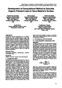
4.2. S TATISTICAL UNCERTAINTY
37
Figure 4.3: Schematized version of the Westkapelle dike-foreshore system, with the stochastic variables indicated by their tags.
4.2. S TATISTICAL UNCERTAINTY According to Van Gelder (2000), statistical uncertainty occurs when the parameters of a distribution are determined with a limited number of data, The smaller the number of data, the larger the parameter and distribution type uncertainty. Because the influence of the statistical uncertainties was considered small, they were not included in this study, as well as to keep the total amount of stochastic variables and thus calculation times reasonably small.
4.3. M ODEL UNCERTAINTY According to Van Gelder (2000), many of the models describing for instance wind and waves are imperfect, caused by omitting variables of lesser importance for reasons of efficiency or because the physical phenomena are not known. The parameters indicating model uncertainty are given below.
4.3.1. B REAKER INDEX The wave breaker index (γ), which affects high frequency waves and low frequency generation, was taken as normal distributed. The mean value stems from the preferred WTI 2017 settings for XBeach (see table 5.1), the standard deviation was taken from Roelvink (1993), in which a calibrated formulation for the dissipation of short-wave energy was derived. It has to be noted that the parameter described here concerns the XBeach breaker index parameter (see e.g. Deltares (2015b)), which has a different definition than the breaker index in Battjes and Janssen (1978). The XBeach parameter is based on Roelvink (1993), with one difference with the original formulation being that the wave dissipation is considered proportional to H 3 /h instead of H 2 . 4.3.2. WAVE SKEWNESS & ASYMMETRY A discretization of the wave skewness (FacSk) and asymmetry (FacAs) was introduced by Van Thiel de Vries (2009), to affect the sediment advection velocity and foreshore morphodynamics. This formulation is also included in XBeach. The mean values of the calibration factors for wave skewness and asymmetry were taken from the WTI 2017 settings for XBeach. Not much information is available on these factors, so some variation (a standard deviation of 0.10) was taken around the mean values. Because negative values of these factors are not possible, the normal distributions were changed into lognormal distributions, using the method de-
38
C HAPTER 4. PARAMETERS & U NCERTAINTIES
scribed in Appendix F.
4.3.3. E UR OTOP COEFFICIENTS The values of the normal distributions of the EurOtop coefficients C 1 and C 2 for ξ< 5, C 3 for ξ> 7 and C 4 for zero freeboard, which all affect the wave overtopping discharge, are presented in EurOtop (2007).
4.4. I NHERENT UNCERTAINTY: TIME According to Van Gelder (2000), when determining the probability distribution of a random variable that represents the variation in time of a process, there is essentially a problem of information scarcity.
4.4.1. S TORM DURATION The distribution of the storm duration was taken from the Hydra-K project and software package (RIKZ, 2006), which recommends a normal distribution with a mean of 54.3 hours and a standard deviation of 18.8 hours, which is then converted into a lognormal distribution, using the method as presented in Appendix F. A maximum storm duration was set at 200 hours, to save computational time. 4.4.2. WATER LEVEL The distributions for the hydraulic boundary conditions were taken from Deltares (2007), in which a probabilistic dune erosion method was developed. Deltares (2007) in turn, used the statistics in the so-called stations or ‘steunpunten’ from the Dutch hydraulic boundary conditions framework (Hydraulische Randvoorwaarden) HR 2006, which provided a list of boundary conditions for each dune profile along the Dutch coast, e.g. (Deltares, 2004). The omni-directional statistics in the stations are valid for the -20 m+NAP depth contour to the North of the Maasvlakte, and valid for a location past the most offshore breaker zone to the South of the Maasvlakte. In these statistics, the water level, significant wave height and wave peak period are correlated, as is further explained below. A conditional Weibull distribution is recommended for the maximum water level reached during a storm (RWS/RIKZ, 2000). This conditional Weibull distribution is described by: £ ¤ F e (H > h) = ρ exp −(h/σ)α + (ω/σ)α (4.1) where h is the highest water level during a storm [m], F e is the frequency of exceedance of the highest level h [year-1 ], α is a shape parameter that depends on the location along the coast, ω is a threshold above which the function is valid, σ is a scale parameter that depends on the location along the coast and ρ is the frequency of exceedance of the threshold level ω. This equation gives the frequency of exceedance, to convert this into the probability of exceedance, the following equation is used: P e (H > h) = 1 − exp [−F e (H > h)]
(4.2)
The parameters of the conditional Weibull distribution are given for different for locations along the North Sea Coast in the stations or ‘steunpunten’. The parameters for the different stations are presented in table 4.2. Table 4.2: Conditional Weibull parameters for Dutch Coast stations (Deltares, 2007).
Location (station)
ω [m]
ρ [year-1 ]
α [-]
σ [m]
Vlissingen Hoek van Holland IJmuiden Den Helder Eierland Borkum
2.97 1.95 1.85 1.6 2.25 1.85
3.907 7.237 5.341 3.254 0.5 5.781
1.04 0.57 0.63 1.6 1.86 1.27
0.2796 0.0158 0.0358 0.9001 1.0995 0.535
4.4.3. WAVE HEIGHT For a given surge level according to the distribution described above, different wave heights can occur, due to the effects of wind speed, wind direction and wind duration. It was found that this correlation could be approximated by a normal distribution with a mean of 0 and a standard deviation of 0.6 m (Deltares, 2004).
4.4. I NHERENT UNCERTAINTY: TIME
39
In the HR 2006 framework (Deltares, 2004), the relation between surge and wave height has been determined as: H s = a + bh − c(d − h)e (4.3a) which is valid for the interval NAP+3 m< h< d . For h> d , the following equation can be used: (4.3b)
H s = a + bh
where a, b, c, d and e are statistical parameters, again given for the different stations. They can be found in table 4.3. To prevent negative wave height values from occurring, a minimum wave height value was set at 0.5 m. Table 4.3: Parameters relation mean wave height and maximum water level (Deltares, 2007).
Location (station)
a [m]
b [-]
c [-]
d [m]
e [-]
Vlissingen Hoek van Holland Ijmuiden Den Helder Eierland Borkum
2.4 4.35 5.88 9.43 12.19 10.13
0.35 0.6 0.6 0.6 0.6 0.6
0.0008 0.0008 0.0254 0.68 1.23 0.57
7 7 7 7 7 7
4.67 4.67 2.77 1.26 1.14 1.58
4.4.4. WAVE PERIOD The relation between the wave peak period and the wave height was studied in HKV (2005). A normal distribution with a mean of 0 and a standard deviation of 1.0 s was used for the correlation between wave peak period and wave height. The relation is given as: T p = α + βH s
(4.4)
where α [s] and β [sm-1 ] are parameters that depend on the location along the coast, which are given below in table 4.4. To prevent negative wave period values from occurring, a minimum wave period value was set at 2.5 s. Figure 4.4 shows the probability of exceedance curves for the water level, wave height and wave period. Table 4.4: Parameters relation wave height and wave peak period (Deltares, 2007).
Location (station)
α [s]
β [sm-1 ]
Vlissingen Hoek van Holland Ijmuiden Den Helder Eierland Borkum
3.86 3.86 4.67 4.67 4.67 4.67
1.09 1.09 1.12 1.12 1.12 1.12
4.4.5. WAVE DIRECTIONAL SPREADING Not much information is available on the probability distribution of the wave directional spreading during storms on the North Sea. To gain a first insight, the data of several storms were analysed, amongst which the storm on 28 October 2013 and the storm on 5 December 2013 (also called ‘Sinterklaasstorm’). The data on the wave directional spreading were received from the Rijkswaterstaat Service Desk for the measurement location Europlatform. Because of the shape of the histograms, a normal distribution seemed the most probable, hence a normal distribution was fitted to the data. A Kolmogorov-Smirnov test was used to test the hypothesis that data could be described by this normal distribution, but the distribution had to be dismissed. For a description of the Kolmogorov-Smirnov test, refer to Appendix F. Therefore, the minimum and maximum directional spreading values were taken and a uniform distribution was applied. The data from the Europlatform are given in degrees, to calculate the XBeach JONSWAP directional spreading parameter s, the following formula can be applied: 2 s = 2 −1 (4.5) σ
40
C HAPTER 4. PARAMETERS & U NCERTAINTIES Exceedance curves 12
Value [m or s]
10
Water level [m] Significant wave height [m] Wave peak period [s]
8 6 4 2 0 100
10−1
10−2 10−3 Exceedance probability [1/year]
10−4
10−5
Figure 4.4: Probability of exceedance curves for the hydraulic boundary conditions water level, wave height and wave period at Westkapelle. Based on the HR 2006 for dunes (e.g. Deltares (2007)).
where σ is the directional spreading in radians. More data analysis is required to improve the estimation of the probability distribution of the wave directional spreading during storms.
4.4.6. L OCATION TIDAL PEAK RELATIVE TO SURGE PEAK The from the above resulting maximum surge level, wave height and wave period were used with an updated version of the formulae from, cf. Steetzel (1993), to create a storm profile. The surge profile is composed of a tidal effect and a surge effect. For this thesis, an adjusted version of the formula from, cf. Steetzel (1993) was made, to be able to include a random phase of the tide at the moment of the maximum water level: Ã ¡ ! Ã ¡ ¢ ¢ !2 2π t − T peak π t − T peak ˆ ˆ zs(t ) = h 0 + h a cos + φ + h s cos (4.6) Tt i d e T sur g e where h 0 is the mean water level [m] (here set to zero), hˆ a is the tidal amplitude [m], t the time [s], T peak the time at which the surge is maximum [s], T t i d e the duration of the tide [s], φ the time shift in the occurrence of the maximum tidal water level opposed to the maximum surge level [-], hˆ s is the surge amplitude [m] and T sur g e is the surge duration [s]. The tidal signal at Westkapelle was schematized as a simple M2-tide, with the same amplitude as the in reality occurring maximum spring tide water level, 2.15 m+NAP and a cycle duration of 12.42 hours. No spring-neap tidal cycle was included in the calculations. The storm duration and maximum water level follow from the above described probability distributions. The time difference between the occurrence of the peak of the tide and peak of the surge was schematized as an uniform distribution with values [−2π; 2π]. T peak was set to half the storm duration T sur g e . Because of this and the shape of the surge profile, the maximum surge level occurs at the middle of the storm. This maximum surge level coincides with a random phase of the tide level, because of the uniform distribution of φ. The maximum water level resulting from the conditional Weibull distribution of the North Sea stations is the maximum water level measured in a certain storm with a certain return period at the -20 m+NAP depth contour. This maximum water level is thus the combination of a certain surge and a certain tidal water level, not necessarily the maximum tidal water level. The maximum tidal water level hˆ a and maximum surge level hˆ s need to be entered in formula 4.6. However, only the maximum water level from the conditional Weibull distribution and the maximum tidal level are known. To cope with this, the maximum surge level is first calculated with hW ei bul l −hˆ a and entered into the formula. After that, the tidal level and surge level in time are calculated and the total water level in time is determined. However, due to the fact that, by definition, the maximum water level from the conditional
4.5. I NHERENT UNCERTAINTY: SPACE
41
Weibull distribution occurs at an arbitrary tidal level, the calculated maximum water level during the storm h max =hˆ a +hˆ s is not equal anymore to the conditional Weibull water level. Therefore, the surge level is scaled, by using sc al e = (hW ei bul l −hˆ a )/hˆ s and hˆ s scal ed =hˆ s ∗sc al e. Then, the surge level, tidal level and total water level in time are again calculated. Now, the maximum water level during the storm agrees with the level from the conditional Weibull distribution and consists of a certain surge and a certain tidal level, which is not necessarily the maximum tidal level. The variation of the significant wave height during the storm was modelled by H s (t ) = Hˆ s cos2
à ¡ ¢! π t − T peak
(4.7)
3T sur g e
in which H s is the significant wave height [m] at time t [s] and Hˆs is the maximum significant wave height (from equation 4.3) [m]. The wave peak period was then modelled, viz. T p (t ) = Tˆp cos
à ¡ ¢! π t − T peak
(4.8)
3T sur g e
where T p is the wave peak period [s] at time t [s] and Tˆp is the maximum wave peak period (from equation 4.4) [s]. An overview of the resulting hydraulic boundary conditions for an arbitrary situation is presented in figure 4.5.
Hm0 [m]
η [m]
4 2 0
5.5 5 4.5 4 3.5
0
5
10
15
20
25
30
35
40
45
50
55
0
5
10
15
20
25
30
35
40
45
50
55
0
5
10
15
20
25
30
35
40
45
50
55
Tp [s]
10 9 8
time [hours] Figure 4.5: Hydraulic boundary conditions during a storm. Water level, significant wave height and wave peak period. Tidal peak coinciding with surge peak. Divided into one hour sections. Storm shape based on Steetzel (1993).
4.5. I NHERENT UNCERTAINTY: SPACE According to Van Gelder (2000), when determining the probability distribution of a random variable that represents the variation in space of a process, there is essentially a problem of shortage of measurements.
4.5.1. D IKE PARAMETERS As mentioned earlier, the dike at Westkapelle was schematized for this thesis. The berm is not included and the average slope is considered, which is tan α = 0.125 or 7.13°. According to TNO (1999), the dike slope is normal distributed, with a coefficient of variation of V = 0.05. According to the same source, the crest height is normal distributed, with a standard deviation of 0.1. As mentioned before, the mean crest height of the Westkapelle sea defence was taken as the crest height in the schematization for this thesis, being 12.6 m+NAP.
42
C HAPTER 4. PARAMETERS & U NCERTAINTIES
4.5.2. S EDIMENT SIZE AND BED FRICTION The sediment size D 50 was determined from Van de Graaff et al. (2007) as being approximately 300 µm and is lognormal distributed with a coefficient of variation of 0.15, according to TNO (1999). The D 90 was then calculated by taking 1.5 times the D 50 . Not much information about the Manning friction factor is available for this location. Therefore, the preferred value of 0.02 was taken from Deltares (2015b) with some spreading around it, which results in the uniform distribution with lower and upper limits of 0.01 and 0.03.
4.6. LSF In general, the limit state function (LSF) that is used for wave overtopping is defined as Z = q cr i t − q, with q cr i t a critical wave overtopping discharge depending on the type of layer and quality of the layer on the inner slope of the dike. For Westkapelle, this limit is 0.1 ls-1 m-1 . Sometimes, the deterministic value of the critical wave overtopping discharge is assumed to also contain uncertainty. This was not used here, because of efficiency reasons. A changing critical wave overtopping discharge increases the difficulty of finding a good ARS fit with ADIS. The shape of the standard wave overtopping LSF is shown in figure 4.6. This function shows a constant value of Z = q cr i t for a large part of the wave heights and then suddenly drops very fast below zero. It was determined that ADIS has difficulties with finding a ARS which fits this function. Therefore, the LSF that was used for this thesis, was changed into Z = log(q cr i t ) − log(q), which has a much smoother shape, see figures 4.6 and 4.7. For the situation as described in section 3.4.1, the amount of calculations necessary for these two limit state functions was 342 exact evaluations for the standard wave overtopping LSF versus 70 exact evaluations for the LSF with the logarithm. However, a disadvantage of this LSF is that it becomes infinity if q becomes 0. Therefore, a minimum value of q= 10−99 ls-1 m-1 was set. Such discontinuities cause problems when using FORM, which was also one of the reasons that ADIS was chosen. Zoom: Hm0 vs z
Hm0 vs z (Tm-1,0=10, slope=0.125, Rc=8, qcrit=0.1)
0.2
10
0.1 z [l/s/m]
z [l/s/m]
5
0
−10
0
2
4
6
z=qcrit-q z=log(qcrit)-log(q) z=0 line
−0.1
z=qcrit-q z=log(qcrit)-log(q) z=0 line
−5
0
−0.2 8
10
Hm0 [m] Figure 4.6: Wave overtopping limit state functions.
0
2
4
6
Hm0 [m] Figure 4.7: Zoom of wave overtopping limit state functions.
4.7. S UMMARY & C ONCLUSIONS This chapter aimed to provide an answer to sub-question 3: the probability distributions that describe the important parameters, and the parameters with the largest influence on morphological change, wave height, wave period and wave overtopping. The first part was answered in this chapter, the second part will be answered in chapter 6.
4.7.1. C HOICE OF PARAMETERS 17 parameters were chosen according to expert judgement and categorized according to Van Gelder (2000), as shown in table 4.1. Statistical uncertainties were not considered, in order to keep the total amount of vari-
4.7. S UMMARY & C ONCLUSIONS
43
ables small and because the influence was deemed small. Under model uncertainty, the breaker index, the calibration factors for wave skewness and wave asymmetry and four EurOtop coefficients were chosen. In the category inherent uncertainty in time, the storm duration, water level, wave height, wave period, wave directional spreading and the moment in time of the tidal peak relative to the surge peak were chosen. The distributions of water level, wave height and wave period were chosen according to the HR 2006 for dunes, which relates these parameters to one another. The storm profile in time was schematized according to Steetzel (1993). Parameters that represent inherent uncertainty in space were the dike parameters crest height and outer slope, and the sediment size and Manning bed friction factor.
4.7.2. L IMIT STATE FUNCTION Due to the shape of the standard wave overtopping LSF, the function was changed to Z = log(q cr i t ) − log(q), which has a much smoother shape. Sometimes, the critical wave overtopping discharge q cr i t is also chosen as a stochastic variable. This was not done here, for the same reason as the change in LSF, because of the increased difficulty for ADIS to fit a good adaptive response surface.
5 A PPLICATION OF MODELS
Sub-question 1 Hydrodyn. & Morph. model
Chapter 2 Literature study
Chapter 3 Model approach & Selection of models
Sub-question 2 Probabilistic model
Chapter 4 Parameters & Uncertainties Chapter 5 Application of models
Chapter 6 Sensitivity analysis
Chapter 7 Uncertainty analysis
Sub-question 4 Infragravity waves
Sub-question 3 Parameters & Distributions
Sub-question 5 Morphological change
Chapter 8 Discussion
Chapter 9 Conclusions & Recommendations
Figure 5.1: Outline of this report.
45
Sub-question 6 Simplification framework
46
C HAPTER 5. A PPLICATION OF MODELS
In this chapter, it is described how the models that were chosen in chapter 3 are applied in the probabilistic framework of ADIS, XBeach and EurOtop. Thus, this chapter aims to provide an answer to parts of the first and second sub-question. The first sub-question was: What method is appropriate to calculate the morphological changes of the foreshore, the infragravity waves and wave overtopping during a storm? The second sub-question was: With what kind of probabilistic framework can the probability of dike failure due to wave overtopping, influenced by a sandy, erodible foreshore be calculated? This chapter describes the settings that were used for the different models, and also presents a validation of XBeach. Section 5.1 gives an introduction to the chapter and set-up of the framework. In section 5.2, the XBeach models that were used for the calculations are described. Section 5.3 describes the determination of the wave spectra at the toe of the dike. Next, section 5.4 shows the calculation of the wave overtopping discharge and 5.5 presents the ADIS settings that were used. After that, in section 5.6 a validation of XBeach was performed by comparison to experiments of Van Gent (1999). Finally, in section 5.7 a summary and conclusions to the chapter are presented.
5.1. I NTRODUCTION
47
5.1. I NTRODUCTION The models that were chosen in chapter 3 need to be combined to be able to calculate the probability of dike failure due to wave overtopping. The combination and application of the models is described in this chapter. The combination of models leads to a framework or ‘model train’, as shown in figure 5.2. In the framework, ADIS determines the random variables. The calculation is started and a random direction and samples are determined. After that, using the samples from the random variables, XBeach calculates the wave transformation (and when enabled the morphological changes) in the dike-foreshore system and gives several parameters at the toe of the dike. Next, for each hour of the storm, the wave spectra at the dike toe are calculated and from that the spectral wave period (Tm−1,0 ) and wave height (Hm0 ) at the dike toe are determined. This wave heights and wave periods are entered into the EurOtop formulae, which calculates the wave overtopping discharge for each hour of the storm. The wave overtopping discharges during the storm are compared and the largest one is chosen. ADIS then calculates the Z -value, hence the result of the limit state function. When the converged probability of failure is found, the calculation is stopped. Otherwise, the process is repeated with a new random direction and new samples from the random variables. When a good fit for the ARS is found, analytical calculations using the ARS are used instead of XBeach calculations, which reduces the computation duration. However, still a small amount of ‘exact’ XBeach calculations will be needed to maintain precision. Probabilistic method: ADIS Random direction & samples Wave transformation (& foreshore deformation): XBeach Parameters at dike toe Wave parameters: Calculation of wave spectra Hm0 , Tm−1,0 at dike toe New calculation or random direction
Wave overtopping discharge: EurOtop q
Z -value: ADIS
Estimate of P f
no
P f converged?
yes
Stop
Figure 5.2: Modelling framework or ‘model train’, using ADIS, XBeach and EurOtop to calculate the probability of dike failure due to wave overtopping.
48
C HAPTER 5. A PPLICATION OF MODELS
5.2. XB EACH CALCULATIONS For the XBeach calculations, the surf-beat version of XBeach was used. The models that were used, included the long waves, the short waves on the wave group scale, flow, sediment transport and morphology. Two different types of models were used, a 1D model and a ‘semi-2D’model, in which no alongshore variations in the profile were included. For the calculations in this thesis, the Westkapelle sea defence was schematized based on the 2009 JARKUS transect 1832, see figures 1.5 and 1.6. Instead of the local crest height at transect 1832, the mean crest height of the Westkapelle sea defence was used, being 12.6 m+NAP. Furthermore, the dike was shchematized without the berm and the bathymetry was simplified to two line sections, to be able to easily include different foreshore shapes and sizes, and to be able to easily compare a situation without and with a foreshore in future studies. See figure 5.3. The JARKUS profile runs to approximately -10 m+NAP. According to common XBeach practice, the profiles were extended to a depth of -20 m+NAP with a slope of 1:50, to remove boundary effects. As mentioned in the previous chapter, to the South of the Maasvlakte, the hydraulic boundary conditions from the stations (‘steunpunten’) are valid for a point past the most offshore breaker zone. Hence, this is not necessarily -20m+NAP, but the calculations showed that virtually no change in wave height occurs between -20 m+NAP and the most offshore breaker zone. The dike itself was implemented as a hard structure, which means that no erosion of the dike slope was possible. For the 1D- and 2D-models, the cross-shore grid sizes were automatically calculated with the XBeach MATLAB toolbox, which determines these sizes by using the CFL condition. For the 2D-model, in the alongshore direction, a section of 1 km was modelled with grid cell sizes of 50 m. which was created by applying the cross-shore profile everywhere in the alongshore direction, which means that no alongshore variations in the profile were included. An example of a computational grid and bathymetry file for the 2D-model is given in figure 5.4. Westkapelle: JARKUS and schematized profiles 20
JARKUS profile 1832 Schematized profile
Height [m+NAP]
10
0
−10
−20 −1,400
−1,200
−1,000
−800
−600
−400
−200
0
200
Cross-shore distance [m] Figure 5.3: Comparison of JARKUS transect 1832 (2009) and the schematized cross-shore profile.
XBeach uses a coordinate system where the x-axis is always oriented towards the coast and the y-axis is oriented in the alongshore direction. The models used a rectilinear grid with variable grid cell sizes. Furthermore, the MPI version of XBeach was used with the 2D-model, which makes it possible to run XBeach on multiple processor cores, by splitting the computational grid in several sections. This was done in order to save computational time. A comparison between the standard XBeach version and the MPI version showed negligible differences in the results. The 1D model was used for its short calculation duration. The semi-2D approach was chosen because it allows for the inclusion of waves approaching from different directions, good representation of the wave directional spreading, as well as a better representation of the infragravity waves in a 2D model. As is further discussed in Appendix E, with the 1D model, the infragravity waves are not represented as well as with the 2D model, because of the exclusion of the wave directional spreading, which influences the infragravity wave height. However, due to the reasonable results and especially the short calculation durations, the 1D model
5.2. XB EACH CALCULATIONS
49
Figure 5.4: XBeach computational grid and bathymetry for the 2D-model of the schematized Westkapelle sea defence. The 1D-model uses the same cross-shore transect.
was used as well. Where possible, default XBeach settings were used, with the exception of the stochastic model parameters identified in chapters 3 and 6. The settings which differed from the standard XBeach settings, are explained in more detail below. An example of the input files for XBeach, as used for the calculations, is presented in Appendix G. To reduce the computational time with the 2D models, the wave direction was solved at regular intervals using the stationary solver (si ng l e_d i r = 1), which then propagates the wave energy along the mean wave direction. In the stationary solver, the wave energy and roller energy balances are solved line by line, from the seaward boundary in the landward direction. For the in-stationary mode (d t het a) a single directional bin of 120 degrees was used and for the stationary solver (d t het a_s) a smaller bin size of 10 degrees was used. As the solving interval, 60 seconds was chosen. The same settings were used for the 1D XBeach calculations. However, XBeach 1D does not include refraction or wave directional spreading. For the spin-up time of the wave boundary conditions (t aper ), 1200 seconds was chosen. For the offshore and onshore boundaries, absorbing-generating (weakly-reflective) 2D-boundary conditions were included, to reduce boundary effects (abs_2d ), abs_1d in the case of the 1D-model. For the lateral boundaries, cyclic boundary conditions were chosen (c ycl i c = 1), to remove shadow zones with obliquely incoming waves. With the cyclic boundary conditions, the wave energy leaving the lateral boundary on one side can be inserted at the other boundary again. The cyclic boundary conditions can only be used with the MPI version of XBeach, which meant that for the 1D-model, Neumann boundary conditions were used instead. The wind was not used in the models. The wind speed was already incorporated into the boundary conditions of the model (water level, wave height, wave period). Furthermore, a wind stress acting on the water surface inside the model was not used, because the influence was negligible. The keyword r and om = 0 was used, which means that the same set of random numbers was used for each XBeach calculation. According to the new Dutch assessment guidelines (WTI 2017, (Deltares, 2015a)), it is recommended to change a number of default XBeach settings, as shown below in table 5.1. These settings were also used in the XBeach models. The intervals for the output of the global and point variables were set to 1800 and 1 s. No mean output was generated. Global model output was given for 1 variable, the bed level. Point output was given at one point, in the (alongshore) centre of the model, at the toe of the dike. At the toe, the time series output of 4 variables was given; the root-mean-square wave height based on the instantaneous wave energy (H ) (short wave energy), the water level (zs) (this also includes the infragravity waves, the bed level (zb), and the GLM velocity in x-direction (uu). The parameters that were considered as stochastic variables were presented previously in chapter 4.
50
C HAPTER 5. A PPLICATION OF MODELS
Table 5.1: WTI 2017 preferred XBeach settings (Deltares, 2015a). Note that f acSk, f ac As and g amma were used as stochastic parameters. The values from the table were used as mean values in the probability distributions.
Parameter
Default
WTI settings
Description
fw g ammax bet a wet sl p al pha f acSk f ac As g amma
0 2 0.1 0.3 1 0.1 0.1 0.55
0 2.364 0.138 0.26 1.262 0.375 0.123 0.541
Short wave friction coefficient (bed friction) Maximum ratio wave height to water depth (breaking waves) Breaker slope coefficient (wave roller model) Critical bed slope for wet area (avalanching) Wave dissipation coefficient (breaking waves) Effect of wave skewness on sediment transport Effect of wave asymmetry on sediment transport Breaker index (breaking waves)
5.2.1. C OMPARISON JARKUS & SCHEMATIZED BATHYMETRY 2D XBeach calculations without sediment transport or morphological changes were performed with the real JARKUS bathymetry as well as with the schematized profile, the results were compared and agreed reasonably well. The boundary conditions that were used for this comparison were the conditions of the 1/1,000 years storm, deduced from the probability distributions as described in the previous chapter (q.v.). For the 2Dmodel, the wave heights and wave periods at seven locations along the profile were compared and showed similar results (see figure 5.5 and figure 5.6), with the largest difference in wave height occurring along the foreshore slope, being 0.35 m, and the largest difference in wave period occurring at the dike toe and being 1.2 s. The differences were much smaller along the rest of the profiles, due to which the representation of the schematized profile was deemed sufficient. JARKUS versus schematized profile, Tm-1,0
Data points along cross-shore 6
Wave period schematized [s]
Significant wave height schematized [m]
JARKUS versus schematized profile, Hm0
4
2
0
0
2
4
20
15
10
6
10
Significant wave height JARKUS [m] Figure 5.5: Comparison between wave heights for XBeach calculations with JARKUS transect 1832 bathymetry and schematized bathymetry.
Data points along cross-shore
15
20
Wave period JARKUS [s] Figure 5.6: Comparison between wave periods for XBeach calculations with JARKUS transect 1832 bathymetry and schematized bathymetry.
5.3. C ALCULATION OF THE WAVE SPECTRA AT THE TOE The time series of model data at the toe of the dike were loaded into MATLAB. The de-trended water depth data can be used to calculate the low frequency (infragravity) wave height and period. The GLM velocity in x-direction and water depth were used to separate the incoming from the reflected waves. The water depth is calculated by subtracting the bed level from the water level. The spectra can be calculated on the basis of the incoming waves only or the incoming and reflected waves. For this thesis, only the incoming waves were used, because the physical model tests on which the EurOtop formulae are based also only included the incoming waves. To separate the incoming and reflected waves, a method based on Van Thiel de Vries (2009)
5.3. C ALCULATION OF THE WAVE SPECTRA AT THE TOE
51
was used, which was in turn based on Guza et al. (1984): ηi n =
ηc out +Q c i n + c out
(5.1)
η out =
ηc out −Q c i n + c out
(5.2)
where ηi n and ηout [m] are the surface elevations associated with the incoming and reflected waves and Q= uh, with u the velocity [m/s] and h the water depth p [m]. Because of the limited water depth at the toe, it is assumed that the outgoing waves travel with c out = g h. For the velocity of the incoming waves, the actual wave group velocity is used: c i n =c g (based on the Tm−1,0 wave period). Next, the data was split into sections during which the boundary conditions were approximately constant (set to 1 hour). For each section, the low frequency spectrum was calculated by taking the resulting data of the incoming waves only. A linear de-trending method was used for the data. The measurement interval was the same as the resolution of the data, thus 1 s. The frequency resolution was set to 0.005 Hz. The time series was split into smaller overlapping sections, using the Welch method with a maximum overlap of 50%. The Welch method reduces the noise in the estimated spectrum in exchange for reducing the frequency resolution. After the division into segments, the segments were windowed, using a Hann window. The Hann or Von Hann window is given by a cosine function which goes to zero at both ends. For a further description of the Welch method and the Hann window function, refer to Appendix C. In the small scale tests of Van Gent (1999), on which the wave overtopping formula for ξ> 7 was based, the limits of the spectra were set to f mi n = 0.02 and f max = 1.2 Hz. For prototype scale used in this thesis, these limits were scaled with the peak period, which was 1.6 s in the small scale tests and is approximately 10 s in prototype scale, which leads to limits of 0.003 and 0.2 Hz. The high frequency (short wave) wave period and wave height were calculated by using the T p entered in XBeach and by using the H point data, which represents the Hr ms wave height, based on the instantaneous wave energy. XBeach hydrostatic does not calculate the changes in the short wave period. The short wave period [s] is calculated as: Tp (5.3) Tm−1,0 = 1.1 The short wave height [m] is calculated by: Hm0 =
p 2Hr ms
(5.4)
From the short wave period and short wave height, a JONSWAP spectrum and a delta function spectrum were estimated, which were then added to the low frequency spectrum, see figure 5.7. From the resulting total spectra, the total spectral wave period and wave height were calculated, using the moments m k : Z ∞ mk = f k S( f )d f (5.5) f =0
p Hm0 = 4 m 0 m −1 Tm−1,0 = m0
(5.6) (5.7)
The resulting total spectrum based on the low frequency spectrum and the added JONSWAP spectrum, and the spectrum based on the low frequency spectrum with the delta function added were compared for each calculation and showed good agreement.
52
C HAPTER 5. A PPLICATION OF MODELS Determination of wave spectrum 1.4 LF spectrum HF spectrum (estimated JONSWAP) Total spectrum Tm-1,0 total spectrum
Energy density [m2 /Hz]
1.2 1 0.8 0.6 0.4 0.2
0 0.00 0.02 0.04 0.06 0.08 0.10 0.12 0.14 0.16 0.18 0.20 0.22 0.24 0.26 0.28 0.30 Frequency [Hz] Figure 5.7: Low frequency, high frequency and total wave spectrum. The high frequency spectrum uses an estimated JONSWAP shape.
5.4. WAVE OVERTOPPING CALCULATIONS The resulting wave parameters at the toe of the dike, for each period during which the boundary conditions were approximately constant (1 hour) were entered into the EurOtop equations, together with the freeboard, slope of the dike and roughness of the slope, with which the wave overtopping discharge (ls-1 m-1 ) was calculated. Of the resulting overtopping discharges, one for each hour of the storm, the maximum is taken and entered into the limit state function. Because of the use of the omni-directional statistics, the angle of wave incidence is kept at an angle of 0 °to the dike normal, hence 270 °in XBeach.
5.5. ADIS SETTINGS Within ADIS, an accuracy of 95% and a confidence level of 20% were set, which means that the true probability of failure lies with 95% certainty within 20% difference of the calculated probability of failure. These settings were chosen as a trade off between accuracy of the calculated probability of failure and duration of the calculation. For this thesis, the goal is not to calculate the probability of failure with 100% accuracy, but to gain an indication of the order of magnitude of the probability of failure and to compare different probabilities of failure for different situations. Calculating a probability of failure with a very high accuracy is also unnecessary because a schematized version of the Westkapelle sea defence is used. A seed was set for the random number generator, to be able to reproduce results. The default ADIS response surface fitting method was used, together with the default margins of the β-sphere, which means fitting a second order polynomial for the ARS and a β-sphere margin of 0.1. To be able to fit a second order polynomial, a minimum number of LSF evaluations needs to be available, 1 + n + n(n+1) , with n the amount of stochastic variables. The standard 2 start-up method was used, which means that ADIS tries an initial fit with a second order polynomial without cross-terms, which only needs 2n + 1 points. Bisection can be used when no convergence is reached in a certain direction. However, when no convergence is reached with the fitting of the polynomial, it will usually also not be reached with bisection and furthermore, bisection will increase the amount of calculations. Therefore, no bisection was used. The minimum number of sampled directions was set to 50, the maximum set to 1,000. The maximum reliability index value (β) for which ADIS is able to search Z = 0 points in certain directions was set to 8.3, which corresponds to a probability of exceedance of approximately 4 ∗ 10−16 . The minimum number of approximated points was set to 50, such that always a reasonable amount of points are available. The first values that ADIS tries in the probability distributions of the stochastic variables are values corresponding β= 4, which corresponds to a return period that is in the same order of magnitude as the return periods that Dutch legal requirements require for dikes (1/250 - 1/10,000). The value of β= 4 was chosen to reach convergence as fast as possible, because it can be expected that the failure probability also lies in this
5.6. VALIDATION OF XB EACH WITH EXPERIMENTS OF VAN G ENT (1999)
53
order of magnitude.
5.6. VALIDATION OF XB EACH WITH EXPERIMENTS OF VAN G ENT (1999) To check if the (large) wave periods (Tm−1,0 ) at the dike toe resulting from the calculation of the wave spectra were correct, a validation was necessary. Therefore, in order to verify the predictive capabilities of the combination of XBeach and the spectral calculations (Fourier analysis) in MATLAB, the combination of XBeach and Fourier analysis was compared to the flume experiments of Van Gent (1999) (q.v.), on which the EurOtop wave overtopping formula for ξm−1,0 > 7 was based.
5.6.1. D ESCRIPTION EXPERIMENTS VAN G ENT (1999) The experiments consist of physical model investigations in a wave flume to study wave run-up and wave overtopping for situations with shallow foreshores. The shapes of the offshore wave energy spectra, the water depth and the slope of foreshore and structure were varied. The tests were performed in the Scheldt-flume of WL | DELFT HYDRAULICS (now Deltares). The test programme consisted of tests with single and double peaked wave energy spectra, foreshores with slopes of 1:100 and 1:250, structures (dikes) with slopes of 1:2.5 and 1:4 and shallow, intermediate and deep water at the toe of the structure. The foreshores were constructed over a length of 36 m. The distance between the toe of the structure and the wave board was 40 m. Five sets of three wave gauges were placed along the foreshore, of which for this research the set at the toe of the dike was the most relevant. The set-up for the 1:100 slope foreshore and 1:4 slope structure is presented in figure 5.8.
Figure 5.8: Set-up with 1:100 foreshore and 1:4 structure slope, (Van Gent, 1999).
5.6.2. D ESCRIPTION XB EACH MODELS The flume situation was entered into XBeach as a 1D model. As well as in the physical model tests, the structure was not present for the calculation of the wave parameters at the toe and only the incoming waves were considered. Also, the Scheldt-flume includes reflection compensation. Because it was not clear which frequencies could and could not be filtered out in the physical model tests, it was chosen to filter all frequencies and thus only take the incoming waves. The A and C test series with single peaked spectra were reproduced, by using 3 different models: XBeach hydrostatic, XBeach hydrostatic with a lower value of the breaker index g amma and XBeach non-hydrostatic. The results for XBeach hydrostatic will be discussed here, the results of XBeach non-hydrostatic and XBeach with a lower g amma-value are presented in Appendix H. Both the A and C test series use an offshore peak period of 1.6 s and an offshore wave height of 0.141 m. The difference in the series lies in the foreshore and structure slope, 1:100 and 1:4 for the A series and 1:250 and 1:2.5 for the C series. No morphology or sediment transport was used, as the physical model tests were done in a concrete flume. Different values of the bed friction coefficient were considered to model the concrete. Finally, c f = 0.001 was chosen, but a different friction coefficient showed no real influence on the results. As offshore and
54
C HAPTER 5. A PPLICATION OF MODELS
onshore boundary conditions, the 1D absorbing-generating boundary conditions were used. For the lateral boundaries, the ‘wall’ boundary conditions were used, to represent the flume walls. Point output (time series) of wave heights, water levels and velocities was given at the same five locations as the wave gauge arrays in the physical model tests. With these data, the wave spectra were calculated in the same way as described above in section 5.3. Again, only the incoming waves were used, as this was also done for the physical model tests. In order to calculate the wave height and wave period from the spectra, different limits to the spectra were used, because it was not clear which limits Van Gent (1999) used. The plotted spectra in Van Gent (1999) show the frequencies 0.02-1.2 Hz, however in the text it is mentioned that no cut-off was used. Therefore, for the comparison, three different spectral frequency limits were used: 0.02-1.2 Hz, 0-∞ Hz and 1/(10T p )-1.2 Hz. It is also unlikely that Van Gent (1999) included the very low frequency (VLF) oscillations, which range approximately from 10-150 min in prototype scale (Munk, 1950). These waves are standing waves, with a frequency equal to the resonance frequency of the basin, or in this case, flume.
5.6.3. C OMPARISON OF SPECTRA , WAVE HEIGHTS AND WAVE PERIODS The resulting wave heights and wave periods from the calculated spectra at the five locations along the slope were compared, as well as the spectra at the toe of the structure for the A test series. For the C test series, no spectra were available. The wave periods and wave heights along the slope for the A and C test series are presented in the tables in Appendix H, as well as the spectra and all the results for XBeach non-hydrostatic and XBeach with a lowered g amma-value. The tables in the Appendix show the water depth d , wave height Hm0 and wave period Tm−1,0 for the five locations along the slope, with X t oe = 0 being at the toe of the structure. Again, the results of the three different XBeach models are shown, as well as the different frequency limits that were used to calculate the wave parameters from the spectra. The wave spectra at the toe for test series A are presented in figure 5.9, 5.10, 5.11 and 5.12. First off, an important point has to be noted. When the Tm−1,0 wave period is determined from the spectra as given in, cf. Van Gent (1999), different values are found than the ones that are listed in the tables in, cf. Van Gent (1999). Even though the shown spectra range from 0.02-1.2 Hz, this indicates that Van Gent (1999) included frequencies higher than 1.2 Hz in the calculation of the Tm−1,0 values. As a result, the Tm−1,0 values that Van Gent (1999) listed in the tables are lower than what would be expected from the spectra in Van Gent (1999). The XBeach Tm−1,0 values were determined from the spectra, with the three different options for the frequency limits. The XBeach hydrostatic spectra show more energy at the peak period, due to the imposed JONSWAP spectrum, but also show less energy in the very high frequency range than the spectra from, cf. Van Gent (1999). Due to the combined effect of these two phenomena, the resulting Tm−1,0 periods for XBeach hydrostatic and frequency limits 0.02-1.2 Hz still agree quite well, even though the shape of the spectra is different. Test A1.03 uses the largest water level, 0.753 m, with the bottom of the flume at 0 m. The spectra at the toe show quite good agreement. Test A1.06 uses the intermediate water level of 0.588 m. Here, XBeach hydrostatic shows a larger energy density in the low frequency range (0.02-0.1 Hz). Near the peak frequency, the hydrostatic model differs considerably from the measurements, because in the hydrostatic model, the spectral transformation of the high frequency wave period is not calculated. Therefore, as described above, a JONSWAP spectrum is superimposed on the low frequency spectrum, which leads to the different spectral shape. Test A1.09 uses a shallow water level of 0.494 m. The spectra agree reasonably well at the lower frequencies, but not at the higher frequencies. Again, the hydrostatic model shows a peak at the peak frequency. Due to this, the XBeach spectrum contains more energy, which leads to a larger wave height than measured in the flume experiments. The low frequency peak of the physical model lies at a somewhat lower frequency than the low frequency peak of the hydrostatic model. Test A1.12 uses a very shallow water level of 0.447 m. Again the peak at the peak frequency in the hydrostatic model is visible (with the accompanying larger wave height), as well as the difference in the location of the low frequency peaks, although they contain approximately the same energy density. Because the wave period Tm−1,0 is heavily influenced by these low frequencies a difference in the location of these peaks could lead to (large) differences in the wave period. Table 5.2 shows the differences between the flume experiments and the XBeach hydrostatic model with frequency limits 0.02-1.2 Hz in significant wave height and wave period at the toe of the structure. In general, the wave height and wave period are represented quite well by the different models. It has to be noted that at the most offshore location, there is already a deviation in the wave height, but not in the wave period (see the tables in Appendix H). This deviation could indicate boundary problems caused by the schematization of the flume in XBeach. At the toe, in general, the frequency limits of 0.02 and 1.2 show the best results.
5.6. VALIDATION OF XB EACH WITH EXPERIMENTS OF VAN G ENT (1999)
55
The wave height at the toe shows small differences with the different frequency limits, but the wave period is influenced more severely, which can be explained by considering the definition of the Tm−1,0 wave period (the first negative moment), which indicates a large influence of the energy in the low frequencies. Of the different XBeach models, in general, the non-hydrostatic model reproduces the shape of the spectra the most accurately, but the hydrostatic model produces the most accurate wave heights and periods. The differences are largest for the tests with the lowest water depth (A1.12 and C1.12). For such small water depths and thus low amounts of wave energy, a small error in the wave spectrum already leads to a significant deviation in wave height and wave period. The absolute differences in wave height are generally small. The differences in wave period are also small, with the largest differences occurring for the A1.12 and C1.12 test. When the relative differences are considered, the errors seem larger, however, it has to be considered that a very small difference of 0.012 m in the C1.12 test, together with a wave height at the toe of only 2.4 cm, already leads to a large relative difference, due to this very small wave height. In general, the differences between the physical model tests and XBeach hydrostatic with limits 0.021.2 Hz are reasonably small. The low frequency waves can be of influence on the wave overtopping, so it is recommended to study the influence of these low frequency waves on wave overtopping in more depth. Because the standard hydrostatic model and the frequency limits of 0.02-1.2 Hz perform the best, these were chosen for the remainder of this thesis. In the figures 5.9-5.12 the XBeach Tm−1,0 periods calculated with frequency range 0.02-∞ Hz are shown together with the Tm−1,0 periods as presented in Van Gent (1999), but in the calculations with the model framework, the 0.02 - 1.2 Hz frequency limits will be used, which become 0.003-0.2 Hz when scaled to prototype scale (by scaling with the peak period). Using these limits instead of 0.02-∞ Hz gives a difference in Tm−1,0 ≤4% in prototype scale, due to the underestimation of the very high frequency energy in XBeach. A (maximal) difference of 4% in Tm−1,0 can result in a maximum difference of about 1% in q, so the influence of the underestimation of the very high frequency energy in XBeach is limited. When using the limits of 0.02-1.2 Hz, for the model tests with deep water the wave period is somewhat overestimated, and for the tests with shallow water the wave period is somewhat underestimated. These differences can be explained by the definition of the Tm−1,0 wave period, in which the low frequencies have a very large influence, as well as the differences in the spectral shapes as explained before. Clear rules should be determined for calculating the Tm−1,0 wave period when infragravity waves are present, because this wave period is so sensitive to the low frequencies. The resulting wave parameters were very sensitive to changes in the frequency resolution with which the spectrum was calculated, as well as the frequency limits. As mentioned above, the frequency resolution was set at 0.005 Hz, based on expert judgement, but the determination of the frequency resolution and frequency limits for deriving the Tm−1,0 period is thus a topic for further research. Table 5.2: Relative differences in wave height and wave period at the toe of the structure between flume experiments (cf. Van Gent (1999)) and XBeach hydrostatic, with frequency limits 0.02-1.2 Hz. Offshore significant wave height 0.141 m, offshore wave peak period 1.6 s. Mean absolute difference in wave height 15.8%, mean absolute difference in wave period 9.1%.
Test
Measured Hm0 [m]
Modelled Hm0 [m]
Difference in Hm0 [%]
Measured Tm−1,0 [s]
Modelled Tm−1,0 [s]
Difference in Tm−1,0 [%]
A1.03 A1.06 A1.09 A1.12 C1.03 C1.06 C1.09 C1.12
0.134 0.104 0.057 0.036 0.132 0.099 0.050 0.024
0.130 0.099 0.066 0.045 0.127 0.097 0.060 0.036
-4% -3% +15% +26% -4% -3% +20% +51%
1.59 1.89 3.20 7.33 1.64 2.17 2.85 4.27
1.68 2.20 3.26 5.58 1.80 2.19 2.75 3.87
+6% +17% +2% -24% +10% +1% -4% -9%
5.6.4. C ONCLUSIONS OF VALIDATION Some general conclusions that can be drawn from the above are: • Even though the spectra from Van Gent (1999) range from 0.02-1.2 Hz, Van Gent (1999) included frequencies higher than 1.2 Hz in the calculation of the Tm−1,0 values. As a result, the Tm−1,0 values that
56
C HAPTER 5. A PPLICATION OF MODELS Van Gent (1999) listed in the tables are lower than what would be expected from the spectra. • Near the peak frequency the hydrostatic model differs from the measurements, because the hydrostatic model does not calculate the transformation of the high frequency wave period. The XBeach hydrostatic spectra also show less energy in the very high frequency range than the spectra from Van Gent (1999). Due to the combined effect of these two phenomena, the resulting Tm−1,0 periods for XBeach hydrostatic still agree quite well, even though the shape of the spectra is different. XBeach (hydrostatic) needs to be improved to be able to also predict the spectral shape in a correct way. • The low frequency peaks contain approximately the same amount of energy, but are located slightly different. • The wave period Tm−1,0 is heavily influence by the low frequencies, frequency resolution and frequency limits, which can easily lead to (large) differences in the wave period. It is recommended to determine clear guidelines on how to determine the Tm−1,0 wave period when infragravity waves are present. • At the most offshore location (near the wave board), there is already a deviation in wave height, but not in wave period. This could indicate boundary problems or could be a model artefact from XBeach, but this needs to be investigated in more detail. • It is recommended to study the influence of low frequency waves on wave overtopping in more depth. • The from the wave spectra resulting wave parameters were heavily influenced by the frequency resolution with which the spectrum was determined. The determination of the frequency resolution remains a topic for further research. • XBeach hydrostatic with frequency limits 0.02-1.2 Hz showed the best results and will be used in the remainder of the thesis. When converted to prototype scale, these limits become 0.003-0.2 Hz.
5.6. VALIDATION OF XB EACH WITH EXPERIMENTS OF VAN G ENT (1999)
Van Gent versus XBeach: A1.03 ·10−2
6
Van Gent Tm-1,0 VG XB hydrostat. Tm-1,0 XB
0.8
Energy density [m2 /Hz]
Energy density [m2 /Hz]
1
0.6 0.4 0.2 0
0.2
0.4
0.6
0.8
1
57
Van Gent Tm-1,0 VG XB hydrostat. Tm-1,0 XB
4
2
0
1.2
Van Gent versus XBeach: A1.06 ·10−3
0.2
Frequency [Hz]
Energy density [m2 /Hz]
Energy density [m2 /Hz]
8
Van Gent Tm-1,0 VG XB hydrostat. Tm-1,0 XB
1
0.5
0
0.2
0.4
0.6
0.8
0.8
1
1.2
Figure 5.10: Spectra for test A1.06, cf. (Van Gent, 1999). Note that the wave periods as shown were calculated with frequency limits 0-∞ Hz. Note that the vertical axis is varying per plot.
Van Gent versus XBeach: A1.09 ·10−3
1.5
0.6
Frequency [Hz]
Figure 5.9: Spectra for test A1.03, cf. (Van Gent, 1999). Note that the wave periods as shown were calculated with frequency limits 0-∞ Hz. Note that the vertical axis is varying per plot.
2
0.4
1
Frequency [Hz] Figure 5.11: Spectra for test A1.09, cf. (Van Gent, 1999). Note that in this figure the wave periods almost coincide, which is why it seems like only one dashed line is plotted. Note that the wave periods as shown were calculated with frequency limits 0-∞ Hz. Note that the vertical axis is varying per plot.
1.2
Van Gent versus XBeach: A1.12 ·10−4 Van Gent Tm-1,0 VG XB hydrostat. Tm-1,0 XB
6
4
2
0
0.2
0.4
0.6
0.8
1
Frequency [Hz] Figure 5.12: Spectra for test A1.12, cf. (Van Gent, 1999). Note that the wave periods as shown were calculated with frequency limits 0-∞ Hz. Note that the vertical axis is varying per plot.
1.2
58
C HAPTER 5. A PPLICATION OF MODELS
5.7. S UMMARY & C ONCLUSIONS This chapter aimed to provide an answer to parts of the first and second sub-question: the best fit morphological, hydrodynamic, wave overtopping and probabilistic methods to determine the probability of dike failure due to wave overtopping. The models that were chosen in chapter 3 were applied in this chapter, to be able to eventually determine the probability of failure in chapter 7.
5.7.1. A PPLICATION OF XB EACH The XBeach hydrostatic models that are used for the calculations, include the long waves, the short waves on the wave group scale, flow, sediment transport and morphology. The MPI version of XBeach was used in combination with cyclic boundary conditions. A semi-2D model was used, with a rectilinear grid with variable grid cell sizes. The profiles in the cross-shore direction were based on the JARKUS profiles at Westkapelle, where the dike was schematized without the berm and in which the bathymetry was simplified to two line sections. In the alongshore direction, a section of 1 km was modelled with grid cell sizes of 50 m. No alongshore variations in the cross-shore profile were included. The wave heights and wave periods at several locations along the profile were compared to the real JARKUS bathymetries at Westkapelle and showed similar results. 5.7.2. C ALCULATION OF SPECTRA The from the XBeach calculations resulting time series at the toe of the dike were loaded into MATLAB. Only the incoming waves were used in the determination of the spectra. For each hour of data, during which the boundary conditions were regarded as being constant, two spectra were calculated, one low frequency spectrum with a high frequency JONSWAP spectrum added to it, and one low frequency spectrum with a high frequency delta function added to it. These spectra showed good agreement. For the frequency resolution 0.005 Hz was used, for the spectral limits 0.003-0.2 Hz. From these spectra the wave height (Hm0 ) and wave period (Tm−1,0 ) at the dike toe were determined. 5.7.3. C ALCULATION OF WAVE OVERTOPPING DISCHARGE The resulting wave parameters were entered into the EurOtop equations, together with the freeboard, main wave direction, slope of the dike and roughness of the slope, with which the wave overtopping discharge was calculated. 5.7.4. P ROBABILISTIC SETTINGS Within ADIS, an accuracy of 95% and a confidence level of 20% were set. The default ADIS response surface fitting method was used, together with the default margins of the β-sphere. The minimum number of sampled directions was set to 50, the maximum set to 1,000. 5.7.5. VALIDATION OF XB EACH In some cases, large wave periods (Tm−1,0 ) at the dike toe resulted from the calculation of the wave spectra with the combination of XBeach and Fourier analysis. Therefore, this combination was compared to the flume experiments of Van Gent (1999), on which the EurOtop wave overtopping formula for ξm−1,0 > 7 was based. From this comparison, it could be concluded that the wave height and wave period are represented reasonably well. The differences in the Tm−1,0 wave periods were caused by the very heavy weighing low frequencies in the calculation of this wave period, as well as differences in the shape of the spectra. Small differences in the low frequency energy between the flume experiments and XBeach can already lead to large differences in the Tm−1,0 wave period. Furthermore, it was determined that the resulting wave parameters at the toe are very sensitive to changes in the frequency resolution with which the wave spectrum is determined, which is a topic for further research. Finally, XBeach hydrostatic with spectral frequency limits of 0.02-1.2 Hz (in model scale) were chosen for further use in this thesis, because this combination showed the best results.
6 S ENSITIVITY ANALYSIS
Sub-question 1 Hydrodyn. & Morph. model
Chapter 2 Literature study
Chapter 3 Model approach & Selection of models
Sub-question 2 Probabilistic model
Chapter 4 Parameters & Uncertainties Chapter 5 Application of models
Chapter 6 Sensitivity analysis
Chapter 7 Uncertainty analysis
Sub-question 4 Infragravity waves
Sub-question 3 Parameters & Distributions
Sub-question 5 Morphological change
Chapter 8 Discussion
Chapter 9 Conclusions & Recommendations
Figure 6.1: Outline of this report.
59
Sub-question 6 Simplification framework
60
C HAPTER 6. S ENSITIVITY ANALYSIS
This chapter describes the sensitivity analysis, in which the influence of each parameter, that was described before in chapter 4, on the significant wave height and wave period at the dike toe, the bed level change and the wave overtopping discharge is determined. Thus, this chapter aims to provide an answer to part of the third sub-question. The third sub-question was: With which probability distribution can the important parameters be described, and which parameters have the largest influence on morphological change, wave height and wave overtopping? With the results of the sensitivity analysis, the parameters were divided into parameter sets, which were further used in the probabilistic calculations as described in chapter 7. Section 6.1 presents an introduction to the chapter and the sensitivity analysis. The set-up of the analysis is described and the results are shown. Sections 6.2 until 6.6 describe the results of the sensitivity analysis in more detail. Finally, in section 6.7 a summary and conclusions to the chapter are presented.
6.1. I NTRODUCTION
61
6.1. I NTRODUCTION In the sensitivity analysis the influence of each parameter on the wave height, wave period, maximum bed level change and in particular the wave overtopping discharge is examined. The 17 parameters that were described in section 4.1 (q.v.) were considered for the sensitivity analysis. The uncertainty in the actual geometry of the foreshore was not considered in this thesis, hence the profile at the start of the storm was kept the same. For each parameter the mean, 5% and 95% values were taken, except for the offshore conditions (zs, H s , T p ), for which the 1/1,000 years conditions were chosen instead of the mean, and for the location of the peak of the tide, for which 0 and π were taken, which indicates tidal high water coinciding with the peak of the surge and tidal low water coinciding with the peak of the surge. The parameters used in the sensitivity analysis are shown in figure 6.2. The different values for the parameters as used in the sensitivity analysis are shown in table 6.1. Each time, the same 2D XBeach calculation was run, as well as the EurOtop model, with only one parameter altered. These XBeach calculations contained the schematized version of the Westkapelle sea defence as described before in section 3.2 and 5.2. The results are shown in table 6.2 and Appendix I. The Appendix shows the resulting bed level changes in each of the calculations. Because the resulting wave overtopping discharges were very low, the sensitivity analysis was repeated with a lowered crest height, set at 7 m+NAP. These results are shown in table 6.3 and figure 6.3. Off course, with a change in crest height, the wave height, wave period and bed level change stay the same and only the wave overtopping discharge changes. The calculations with the lower crest level show the same trends as the calculations with the standard crest height of 12.6 m+NAP.
Figure 6.2: Stochastic variables as used in the sensitivity analysis.
In the last column of the tables, a division was made according to the importance of the parameters. By doing this, five sets of parameters were created: • Set 1, Offshore conditions: 3 variables, zs, H s , T p . • Set 2, Model and wave parameters: 7 variables, C 1, C 2, C 3, C 4, g amma, n, s. • Set 3, Storm parameters: 2 variables, t st op, l oc_peak. • Set 4, Morphological parameters: 3 variables, D 50 , F ac As, F acSk. • Set 5, Dike parameters: 2 variables, al pha, cr est .
62
C HAPTER 6. S ENSITIVITY ANALYSIS
Table 6.1: Parameter values for the sensitivity analysis. 1/1,000, 5% and 95% values for the offshore conditions, mean, 5% and 95% values for the other parameters.
Description
Parameter
Mean or 1/1,000 years value
Upper bound
Lower bound
Dike slope [-] EurOtop coefficient ξ