A new mixed beta distribution and structural properties with applications

Songklanakarin J. Sci. Technol. 37 (1), 97-108, Jan. - Feb. 2015 http://www.sjst.psu.ac.th

Original Article

A new mixed beta distribution and structural properties with applications Tipagorn Insuk1, Winai Bodhisuwan2, and Uraiwan Jaroengeratikun1* 1

Department of Applied Statistics, Faculty of Applied Science, King Mongkut’s University of Technology North Bangkok, Bang Sue, Bangkok, 10800 Thailand. 2

Department of Statistics, Faculty of Science, Kasetsart University, Chatuchak, Bangkok, 10900 Thailand Received: 27 June 2014; Accepted: 12 December 2014

Abstract In this paper, we introduce a new six-parameter distribution, namely Beta Exponentiated Weibull Poisson (BEWP) which is obtained by compounding between the exponentiated Weibull Poisson and beta distributions. We propose its basic structural properties such as density function and moments for this new distribution. We re-express the BEWP density function as a EWP linear combination, and use this to obtain its moments. In addition, it also contains several sub-models that are well known. Moreover, we apply the maximum likelihood method to estimate parameters, and applications to real data sets show the superiority of this new distribution by comparing the fitness with its sub-models. Keywords: beta exponentiated weibull poisson, beta-g distribution

where ,, > 0 and

1. Introduction For more than a decade, Weibull distribution has been applied extensively in many areas and more particularly used in the analysis of lifetime data for reliability engineering or biology (Rinne, 2008). However, the Weibull distribution has a weakness for modeling phenomenon with non-monotone failure rate. Therefore Mudholkar and Srivastava (1993) proposed the exponentiated Weibull (EW) distribution that is an extension of the Weibull family, obtained by adding a second shape parameter. Then it is flexible to model survival data where the failure rate can be increasing, decreasing, bathtub shape, or unimodal (Mudholkar et al., 1995). Let W be a random variable of the EW distribution. Then the cumulative distribution function (cdf) and probability density function (pdf) of W are given by



F  w   1  e w





,

* Corresponding author. Email address: [email protected]

w  0,

f  w     w 1e

 w 



 1

1  e    w 



, w  0,

respectively. For survival analysis, there are important analytical functions such as survival and hazard rate functions given by



S  w   1  1  e   w 







and h  w     w 1e

  w



 1

1  e  

  w 

    w 1  1  e 





 

1

.

respectively. Recently, many researchers have attempted to modify EW distribution with different techniques by using EW as the baseline distribution to develop more flexibility. Pinho et al. (2012) proposed gamma exponentiated Weibull, Singla et al. (2012) studied beta generalized Weibull (BGW), Cordeiro et al. (2013) introduced the beta exponentiated Weibull (BEW) and exponentiated Weibull Poisson (EWP)

98

T. Insuk et al. / Songklanakarin J. Sci. Technol. 37 (1), 97-108, 2015

was proposed by Mahmoudi and Sepahdar (2013). sub-models of BEWP in the form of table and chart where In this paper, we propose a new flexible six-parameter several sub-models are well known. Section 5 discusses the distribution called Beta Exponentiated Weibull Poisson moment generating function (mgf) and the moment. In (BEWP) distribution. The purpose of this study is to create Section 6 we apply the maximum likelihood method to a new distribution by mixing EWP distribution and the beta estimate parameters, and Section 7 compares the sub-models distribution. Some properties of this new distribution will be of the BEWP distribution by the applications to real data sets. investigated. Some concluding remarks are given in Section 8. The BEWP distribution is developed by using the Beta-G distribution class that was introduced by Eugene 2. The Exponentiated Weibull Poisson distribution et al. (2002) who also proposed the beta normal (BN) distribution. Then, using the Beta-G distribution class was applied Let W1 , W2 , W3 ,..., Wz be independent and identically to create a new distribution extensively. For example, distributed random variables from exponentiated Weibull Nadarajah and Gupta (2004) proposed the beta Frechet (BF) distribution with pdf distribution and Nadarajah and Kotz (2004) studied the beta    1 f  w; ,  ,      w 1e  w 1  e  w , w  0, Gumbel (BGu) distribution. Nadarajah and Kotz (2006) introduced the beta exponential (BE) distribution, Lee et al. and Z, which is independent from W’s, be a random variable (2007) proposed the Beta Weibull (BW), Mahmoudi (2011) from zero truncated Poisson distribution with probability mass proposed the Beta Generalized Pareto (BGP), BGW or BEW function (pmf) and Percontini et al. (2013) studied the Beta Weibull Poisson 1 (BWP). p  z;    e    z  1  z  1 1  e   ,   0, z  1, 2, 3,... The EWP distribution fits the skewed data (Mahmoudi and Sepahdar, 2013) and it is useful for solving complemen- where     is the gamma function. Percontini et al. (2013) tary risks problem (Basu and Klein, 1982) in the presence of described the model for X  min W1 , W2 ,..., Wz  and X = latent risks, in the sense that there is no information aboutX  max W1 , W2 ,...,W z  that can be used in serial and parallel which factor is responsible for the component failure and system with identical components, which appear in many only the maximum lifetime value among all risks is observed. industrial applications and biological organisms. For this Mixing the EWP distribution with the beta distribution causes model, we define X  max W1 , W2 ,...,Wz  . We assume the the two additional shape parameters which serve to control failure occurs after all Z factors have been activated. Then skewness and tail weights of EWP distribution. As a result, we obtain  1  ( z 1) BEWP distribution is the generalized distribution that has g  x z; ,  ,   z  w 1u 1  u  1  u  , x  0, a wide variety in terms of shape of the distribution, so it is  a flexible alternative for applications in engineering and where u  e  x  and the marginal pdf of X is biology. In engineering applications, the BEWP distribution     1  1 can be employed in reliability analysis, such as product relig  x   x u 1  u  e 1u  , x  0, (1) ability and system reliability. Percontini et al. (2013) applied  e 1 the BWP distribution to the maintenance data on active and the cdf of X is repair times for airborne communication. In addition, for  biology or medical science, we may apply to survival analysis e 1u   1 G  x  . (2) e.g. Mudholkar et al. (1996) applied the generalized Weibull e  1 distribution in fitting the real survival time data of the patients Then we take this pdf and cdf of EWP to be the baseline for who were given radiation therapy and chemotherapy from creating the new Beta-G distribution in the next section. We head and neck cancer clinical trial. Dasgupta et al. (2010) apply the interpretation of the EWP from Adamidis and studied the characteristics of coronary artery calcium which Loukas (1998), that the failure (of a device, for example) occurs is a marker of coronary artery disease. This appears to be a due to the presence of an unknown number, Z, of initial Weibull distribution and a Weibull regression model was defects of the same kind (a number of semiconductors from a proposed to examine factors influencing the disease. Ortega defective lot, for instance). The W’s represent their lifetimes et al. (2013) developed the beta Weibull distribution to be and each defect can be detected only after causing failure, the log-beta Weibull distribution and studied the log-beta in which case it is repaired perfectly. Weibull regression model with application to predict recurrence of prostate cancer. 3. The Beta Exponentiated Weibull Poisson distribution The rest of this paper is organized in the following sequence. Section 2 discusses about the exponentiated Definition 1: Weibull Poisson (EWP) distribution that is used as the Let F(x) be the cdf of a random variable X. According baseline to develop the BEWP distribution. The probability to Eugene et al. (2002), the cdf for a generalized class of density function (pdf) and cumulative density function (cdf) distributions can be defined as the logit of beta random are introduced in Section 3. Section 4 gives a summary of variable by









99

T. Insuk et al. / Songklanakarin J. Sci. Technol. 37 (1), 97-108, 2015 hence

G x 

1 B  a, b 

F  x 

b 1

wa 1 1  w  dw, x  0,



(3)

0

where a,b>0. G(x) denotes the probability distribution of the generalized class of distribution. The pdf of X is given by (for more details see Mood et al. (1974)) f  x 

where g  x  

dG  x  dx



 1

e



e



 1u 

 e 1u   1     e  1   





 1 B  a, b 

a 1



 e 1u   1  1    e  1  

b 1



 0

0

f ( x) 

g ( x)  a  i 1  ci  a, b  (a  i)G  x  . B  a , b  i 0

Consider the case where the power of G(x) is a non-integer



 1

  x 1u 1  u 

e

    G  x    ( 1)i   (1  G  x )i i 0 i





e

 1 u 



 1 B  a, b 



 e  1u   1     e  1   

a 1



 e  1u   1  1    e   1  

  i 0 j 0

 f  x  dx    0

1

a 1



v 1   1     e 1 



b 1

dv



G  x  for G  x 

(6)

 j  s j (j +1)( 1)i   e j ,i  1 rj 1 i  and s j  . j  1 B  a, b  (j - i +1) e   1





   i  1 i  j ! j !

j i

j 0 i o

where s j ,i

j

( 1)i  j    1

where d j ( )  

and

ai

, then we substitute

in Eq. (7), we obtain

F  x 

 1 j r j ( a , b )G  x   B  a, b  j 0

f  x 

 1 j g(x) (j +1)rj (a, b)G  x  B  a, b  j 0

j



   i  1 i  j ! j !

j 0

 1. Note that, we can define the expansion of the pdf as the linear combination of EWP density function as

f  x    s j ,i g ( x;  ,  , ,  j ,i )

j

  d j ( )G  x  ,

dx



1  v 1      e  1 B  a, b   e  1 

( 1) i  j    1 G  x 



b 1

let v  e  1 u  , it can be rewritten as e

i







(7)

i stops at b-1. We obtain f(x) for integer a

Simply by using Definition 1, we obtain the pdf of X by substituting g(x) and G(x) from Eqs.(1) and (2) into Eq.(4). Then Eq.(5) is the pdf of BEWP distribution as the following property. f  x  dx  

0

 b  1 (1)i   i   where ci ( a, b)  . If b is an integer, the index a  i

Proof:



  b  1 i wa 1  ( 1)i   w dw i0  i 



 1 a i ci (a, b)G  x  ,  B  a, b  i  0

(5)  x where u  e  

G x 

 b  1 ai (1)i   G  x i 1     B  a, b  i  0 a  i

.

  x  1u 1  u 

1 B  a, b 



b 1 1 a 1 g  x  G  x  1  G  x  , x  0, (4) B  a, b 

Theorem 1: Let X be a random variable of the BEWP distribution with parameters  ,  ,  ,  , a and b. The pdf of X is defined by f  x 

F  x 



where rj ( a, b) 

 c (a, b)d (a +i) or i

j

i 0





j

f  x    s j (j +1)g(x)G  x  , j0

Let b be a non-integer real number and w  1 . 1 F  x  B  a, b 

G x 



b 1

wa1 1  w dw, a, b, x  0

0

By using the special case of binomial theorem

where s j 

rj 1 B  a, b 

and we can express pdf of BEWP dis-

tribution in terms of a linear combination of EWP distribution as 

1  w 

b 1

 b  1 i   (1)  w , i 0  i  

i

    x  1u 1  u  1 e 1u  f  x    s j (j +1)   e  1 j 0 

  e 1u   1      e  1    

j

100

T. Insuk et al. / Songklanakarin J. Sci. Technol. 37 (1), 97-108, 2015  j s j (j +1)( 1)i    i  (j - i+1)  x  1u 1  u  1 e  1u   j i1     j 1  j  0 i  o (j - i+1) e  1 

j







 j  s j (j +1)( 1)i   e j ,i  1 j  i   j 1 j 0 i o (j - i +1) e   1











  

 1

  x  1u 1  u 

j ,i

e

 j ,i



e

  x where u  e  

    

 j ,i 1u 

1

j

Proof: Simply by using Definition 1 again, we can define the cdf of X by replacing G(x) from Eq.(2) in Eq.(3), hence the cdf of BEWP distribution is as obtained in Eq.(8). Note that, we can define the expansion of the cdf as the linear combination of EWP density function given by

  s j ,i g ( x; ,  , ,  j ,i )

F(x)   s j ,i G ( x; ,  , ,  j ,i )

 j  s j (j +1)( 1)i   e j ,i  1 i where  j ,i    j  i  1 and s j ,i  j 1 (j - i +1) e  1









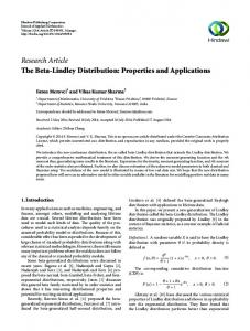
To show the various of shapes of the distribution, some specified parameters of the BEWP distribution and their density functions are provided in Figure 1: (a) Fix parameters  = 4,  = 0.5,  = 1.5,  = 0.5 and vary parameters a and b, and (b) Fix parameters a = 2, b = 2 and vary parameters , ,  and . Thus, the BEWP distribution can be suitable for fitting to various shapes of data, for example where the parameters a = 2, b = 2,  = 4,  = 0.5,  = 1.5,  = 0.5. This distribution is suitable for fitting skewed data and it is suitable for fitting unimodal data when the parameters a = 2, b = 2,  = 0.5,  = 2,  = 0.1,  = 15. According to Figure 1, BEWP distribution can be a family of distributions containing 32 sub-models which will be discussed in Section 4. Theorem 2: Let X be a random variable of a BEWP distribution with parameters  ,  ,  ,  , a and b. The cdf of X is given by 

1 F x  B  a, b 

( e 1u  1)/(e  1)



b 1

wa 1 1  w  dw

(8)

0

or

F  x  I

j



j 0 i o

 1u  ( e   1) /( e 1)

( a,b )

(10)

j  0 i 0

by integrating f(x) in Eq.(6) 

x

j

F(x)   s j ,i  g ( x; ,  , ,  j ,i ) j 0 i 0



j

0

x

  s j ,i  j 0 i 0

 1

 j ,i  x  1u 1  u  e

0

 j ,i

1



e

 j ,i 1u 

dx



 e  j ,i 1u   1     s j ,i   e j ,i  1  j 0 i  0   

j



j

  s j ,iG ( x; ,  ,  ,  j ,i ) j 0 i  0

4. Sub-models This new distribution consists of a total of 32 subdistribution models as shown in Figure 2 and Table 1. In Table 1, the sub-models associated with Poisson distribution, are assigned X  max W1 ,W2 ,..., Wz  which based on the parallel components system comply with BEWP distribution that is under the same assumption. For XX = min W1,W2 ,...,Wz  , we also refer to the References column and mark with the asterisk symbol (*) in Table 1.

(9)

Figure 1. Density function of the BEWP distribution.

101

T. Insuk et al. / Songklanakarin J. Sci. Technol. 37 (1), 97-108, 2015

Figure 2. The sub-model chart of BEWP distribution

Table 1. The sub-model table of BEWP distribution. parameters

Distribution

F(x)

a

b









1. Beta Exponentiated Rayleigh Poisson (BERP)

a

b



2





2. Beta Exponentiated Exponential Poisson (BEEP)

a

b



1





3. Beta Weibull Poisson (BWP)

a

b

1







F ( x)  I

4. Beta Exponentiated Weibull (BEW)

a

b







0

F ( x)  I

5. Beta Rayleigh Poisson (BRP)

a

b

1

2





F ( x)  I

6. Beta Exponential Poisson (BEP)

a

References

5 parameters F ( x)  I

 x

2



) e  (1 e 1 e  1

F ( x)  I

e (1e

 x  ) 

 a, b 

 a, b 

1

e 1

 x



) e  (1 e 1 e  1

 a, b 

Percontini et al. (2013)*

 a, b 

Singla et al. (2012), Cordeiro et al. (2013b)

 x  (1e   )

4 parameters  x 2

) e (1e 1 e 1

b

1

1





F ( x)  I

e (1e

 x  )

1

 a, b 

 a, b 



e 1 

7. Generalized Weibull Poisson (GWP)

a

1

1







 e (1e x )  1   F ( x)    e  1   

8. Exponentiated Weibull Poisson (EWP)

1

1









F ( x) 

a

  x  

e (1e )  1 e  1

Mahmoudi and Sepahdar (2013)

102

T. Insuk et al. / Songklanakarin J. Sci. Technol. 37 (1), 97-108, 2015

Table 1. Continued parameters

Distribution

F(x)

References

a

b









a

1







0

F ( x )  1  e   x 

10. Beta Exponentiated Rayleigh (BER)

a

b



2



0

F ( x)  I

11. Beta Exponentiated Exponential (BEE)

a

b



1



0

F ( x)  I

12. Beta Weibull (BW)

a

b

1





0

F ( x)  I 

9. Generalized Exponentiated Weibull (GEW)



2

(1 e  x  )

 x

 1 e 

3 parameters



1e   

 x 



a





(a,b)

Cordeiro et al. (2013a)

 a, b 

Barreto-Souza et al. (2010)

  

 a, b  a

2

13. Generalized Rayleigh Poisson (GRP)

a

1

1

2





14. Generalized Exponential Poisson (GEP)

a

1

1

1





Lee et al. (2007)

 e (1e x )  1   F ( x)    e  1    a  e  (1e x  )  1  F ( x)     e  1  Barreto-Souza, and   Cribari-Neto (2009)  x 2 

15. Exponentiated Rayleigh Poisson (ERP)

1

1



2





e (1e )  1 F ( x)  e  1

16. Exponentiated Exponential Poisson (EEP)

1

1



1





F ( x) 

e (1e )  1 F ( x)  e  1

Mahmoudi and Sepahdar (2013)

  x  

e (1e )  1 e  1

 x 

17. Weibull Poisson (WP)

1

1

1







18. Exponentiated Weibull (EW)

1

1







0

19. Generalized Weibull(GW)

a

1

1





0

20. Generalized Exponentiated Rayleigh(GER)

a

1



2



0

  F ( x)  1  e 

21. Generalized Exponentiated Exponential(GEE)

a

1



1



0

F ( x )  1  e   x 

22. Beta Rayleigh (BR)

a

b

1

2



0

F ( x)  I 

23. Beta Exponential(BE)

a

b

1

1



0

F ( x)  I 1 e x   a, b 

24. Rayleigh Poisson (RP)

1

1

1

2





F ( x) 

e  (1e )  1 e  1

25. Exponential Poisson (EP)

1

1

1

1





F ( x) 

e (1e )  1 e  1

26. Weibull (W)

1

1

1





0

Percontini et al. (2013)*, Ristiæ and Nadarajah (2014)*, Mahmoudi and Sepahdar (2013) Hemmati et al. (2011)*, Lu and Shi (2012)*, Mahmoudi and Sepahdar (2013)



F ( x)  (1  e x )

F ( x)  1  e

  x 

  x 



 1e 



2 parameters

 x 2

  



Mudolkar and Srivastava (1993) coincide with GW a

Mudolkar and Srivastava (1993) coincide with EW

a

2

Cordeiro et al. (2013a)

a



 a, b 



Nadarajah and Kotz (2006)

2  x 

 x 

Mahmoudi and Sepahdar (2013) Kus (2007)*, Cancho et al. (2011)



F ( x)  (1  e  x  )

Mudolkar and Srivastava (1993)

103

T. Insuk et al. / Songklanakarin J. Sci. Technol. 37 (1), 97-108, 2015 Table 1. Continued parameters

Distribution

F(x)

References

a

b









27. Exponentiated Rayleigh (ER)

1

1



2



0

28. Generalized Rayleigh (GR)

a

1

1

2



0

  F ( x )  1  e 

29. Exponentiated Exponential (EE)

1

1



1



0

F ( x)  (1  e  x  )

30. Generalized Exponential (GE)

a

1

1

1



0

F ( x)  1  e  x 



31. Rayleigh(R)

1

1

1

2



0

F ( x)  1  e  x 



0





32. Exponential(E)

1

1

1

1



F ( x )  1  e   x    x 

5. Moment Generating Function and Moment

a

2



F ( x)  1  e



2

2

 x 

Kundu and Raqab (2005) coincide with GR Kundu and Raqab (2005) coincide with ER Gupta and Kundu (1999) coincide with GE

a

Gupta and Kundu (1999) coincide with EE Johnson et al. (1994)



Johnson et al. (1994)



M X BEWP  t    m t m

Theorem 3: Let X be a random variable of a BEWP distribution with parameters  ,  ,  ,  , a and b. The moment generating function (mgf) of X can be given by 

M X  t    mt m

(11)

m0 j



where m 

m



  i, j, l , m, n      1 and m = 0,1,2,…

j ,l , n  0 i 0

m 0

j



where m 

m

j ,l , n  0 i 0

Theorem 4: Let X be a random variable of a BEWP distribution with parameters  ,  ,  ,  , a and b. The moment of X can be written as n 1

m   m   j s j ,i  l    n  1  1  1 E X m    m    1     j ,i  1    l  1    l   j , n,l 0 i 0 e j ,i  1 n !  

 



Proof: To find the mgf of BEWP distribution, we apply the definition of mgf to the linear combination of EWP density function as 

j



M X BEWP  t    s j ,i  e g  x; ,  , ,  j ,i  dx tx

j 0 i 0

0

j



  s j ,i M X EWP  t ;  ,  ,  ,  j ,i ,



  i, j, l , m, n      1 and m = 0,1,2,…



(12) Proof: To find the moment of BEWP distribution, we apply the definition of moment again to the linear combination of EWP density function as

 



j



EBEWP X m   s j ,i  x m g  x; ,  , ,  j ,i  dx j0 i0

0

j 0 i 0



where Mahmoudi and Sepahdar (2013) derived that M X EWP  t  

 nj ,i t m  m    1 n  0 m 0 l  0 n ! m !

 j ,i e

 j ,i







m  m  l    n  1  1    1     1   1    l  1    . l    





j 0 i 0

where Mahmoudi and Sepahdar (2013) derived that m   n 1 m    l    n  1  1   1  EEWP X m    m    1   j ,i  1    l  1    . j ,i l   n0 i 0 e  1 n !  

 

We can reduce to j



m  M X BEWP  t       i, j, l , m, n     1 t m , j , l , m , n  0 i 0   n 1  m j ,i

m     n  1  1    1   1    l  1    . l  1 n !m !  

 s j ,i  

e

 j ,i



And we can reduce again to be

l





So we can obtain the moment of BEWP distribution as n 1 m   m   j s j ,i  l    n  1  1   1 E X m    m    1    j ,i  1    l  1    . j ,i l   j , n ,l  0 i  0 e  1 n !  

 

where   i , j , l , m, n  

j

  s j ,i EEWP X m ; ,  ,  ,  j ,i ,





Then we can find variance, skewness and kurtosis of random variable X by using the well-known relationship of each moment.

104

T. Insuk et al. / Songklanakarin J. Sci. Technol. 37 (1), 97-108, 2015

6. Parameter Estimation

where   x  

In this section, we suppose that the sample size n was T

drawn from BEWP distribution, and let π   ,  ,  ,  , a, b  be the parameter vector. Then the log-likelihood function of BEWP is given by n



l  ,  ,  ,  , a , b    log    log     log      log    log  B  a, b  

Γ( x) is the digamma function. The maximum Γ( x) T





likelihood estimator πˆ  ˆ , ˆ , ˆ, ˆ, aˆ, bˆ is the solution to the above score equations that are calculated by using Newton-Raphson method in R package (R Core Team, 2012). 7. Applications

i 1









  xi     1 log 1  ui    1  ui    a  1 log e  1ui   1



  b  1 log e  e

   a  b  1 log e 1



 1ui 



  x where ui  e  i  . So the elements of score vector

T

 l l l l l l  U  , , , , ,       a b 

where 

 n   a  1  1  ui  e 1ui  log 1  ui  l 1     log 1  ui     i 1   e 1ui   1 





  b  1  1  ui  e 



log 1  ui     

 1 ui  

e e

 1ui 

 n    1 xi  ui  log  xi   log    l 1      log     xi   log  xi   log      i 1   1  ui 



   xi  ui  log  xi   log    



 1

 a  1  xi  1  ui 



e



 1ui   xi 

 log  x   log    i



e 

 1 ui 

 1

  b  1   xi  1  ui 



1 

e



 1ui   xi 

e e



 log  x   log    i



 1ui 

 

       1 n   1   xi  ui  a  1   xi  1  ui  e 1ui   xi  l     xi         1 u  i 1     1  ui   e  i  1 











 1

  xi  ui   b  1   xi  1  ui      e   e  1ui 





e

 1ui   xi 





    

In this section, to reveal the superiority of BEWP distribution, we fit a BEWP model to two real data sets from the application of EWP (Mahmoudi and Sepahdar, 2013). The first application, we study the skewed data representing strengths of 1.5 cm glass fibers, measured at the National Physical Laboratory, England, which are given in Table 2. Unfortunately, the units of measurement are not given in the paper. For the second application, we examine the data showing the stress-rupture life of Kevlar 49/epoxy strands (unit: hours) which were subjected to constant sustained pressure at the 90 stress level until all had failed as displayed in Table 3. We fit the BEWP distribution to above two data sets and compare the fitness with its sub-models that are BWP, BEW, BEE, EWP, EW, EE including Weibull distribution by considering the p-value of Kolmogorov-Smirnov (K-S) statistics. The maximum likelihood estimates of the parameters, the K-S statistics and the corresponding p-value for the fitted models are shown for data sets I and II in Tables 3 and 4, respectively. Graphical approach is the another way to express these data sets fit with this distribution. We also present the comparison of the empirical cdf wtth each estimated cdf in Figure 3. It shows the fitting of data to proposed models. The probability plots of the BEWP distribution corresponding to data sets I and II in Figure 4 indicate that (a) most data lie around the straight line especially the middle 50% of the data, and (b) the first 75% of the data lie on the straight line and the last 25% of the data lie above, which suggests a slight right-skewness. It seems reasonable to tentatively conclude that both data sets are BEWP distribution. 8. Conclusion



  n   a  11  ui  e 1ui  l 1  a  b  1 e     1  ui      1 u  i1   e 1 e  i  1 

 b  1 

 e  1  u  e 



i



e e



 1ui 

 

Table 2. Strengths of 1.5 cm glass fibers

  



 1 ui 

n  l  1u      a    a  b    log e  i   1  log e  1 a i 1

     l       b    a  b    log  e  e   log e 1  b n



i 1

For this paper, a new six-parameter distribution, namely BEWP is studied. It is obtained by compounding beta



 1 ui 



0.55 1.68 1.53 1.11 1.76 1.61 1.48

0.93 1.73 1.59 1.28 1.84 1.62 1.51

1.25 1.81 1.61 1.42 2.24 1.66 1.55

1.36 2.00 1.66 1.50 0.81 1.70 1.61

1.49 0.74 1.68 1.54 1.13 1.77 1.63

1.52 1.04 1.76 1.60 1.29 1.84 1.67

1.58 1.27 1.82 1.62 1.48 0.84 1.70

1.61 1.39 2.01 1.66 1.50 1.24 1.78

1.64 1.49 0.77 1.69 1.55 1.30 1.89

105

T. Insuk et al. / Songklanakarin J. Sci. Technol. 37 (1), 97-108, 2015 Table 3. Stress-rupture life of Kevlar 49/epoxy strands (unit: hours) 0.01 0.07 0.13 0.36 0.63 0.80 1.02 1.31 1.54 2.02 7.89

0.01 0.07 0.18 0.38 0.65 0.80 1.03 1.33 1.54 2.05

0.02 0.08 0.19 0.40 0.67 0.83 1.05 1.34 1.55 2.14

0.02 0.09 0.20 0.42 0.68 0.85 1.10 1.40 1.58 2.17

0.02 0.09 0.23 0.43 0.72 0.90 1.10 1.43 1.60 2.33

0.03 0.10 0.24 0.52 0.72 0.92 1.11 1.45 1.63 3.03

0.03 0.10 0.24 0.54 0.72 0.95 1.15 1.50 1.64 3.03

0.04 0.11 0.29 0.56 0.73 0.99 1.18 1.51 1.80 3.34

0.05 0.10 0.34 0.60 0.79 1.00 1.20 1.52 1.80 4.20

0.06 0.12 0.35 0.60 0.79 1.01 1.29 1.53 1.81 4.69

Table 4. MLE and K-S statistics with corresponding p-values for the strengths of 1.5 cm glass fibers. Parameters

Fitting Distribution

a

b









BEWP BWP BEW BEE EWP EW EE Weibull

0.1203 0.5032 0.3703 0.4021 -

0.4896 0.8554 3.924 31.4853 -

6.0391 2.3156 24.8020 0.5781 0.6712 31.3485 -

4.9958 5.3956 5.6507 5.5015 7.2845 5.7807

0.7693 0.6782 0.5135 1.0976 0.6466 0.5820 2.6115 0.6142

12.2998 4.6781 2.7821 -

and exponentiated Weibull Poisson distributions. We introduce its basic mathematical properties such as density function. We show that the pdf of BEWP distribution can be expressed in the linear combination form of EWP distribution including its moments. Moreover, it also contains the many sub-models that are well known. Finally, we have applied the maximum likelihood method to estimate parameters and fit the BEWP distribution to two real data sets. We compared the results with its sub-models such as BWP, BEW, BEE, EWP, EW, EE and Weibull distribution. The results showed that BEWP distribution provides a better fit than existing mixtures of the EW or Weibull distribution and some wellknown sub-models. Acknowledgements The authors would like to thank the referees and the editor for valuable comments and suggestions to improve this work. References Adamidis, K. and Loukas, S. 1998. A lifetime distribution with decreasing failure rate. Statistics and Probability Letters. 39, 35–42.

K-S

p-value

0.0705 0.0978 0.1448 0.1999 0.1154 0.1462 0.2291 0.1522

0.9127 0.5827 0.1425 0.0130 0.3713 0.1351 0.0027 0.1078

Barreto-Souza, W. and Cribari-Neto, F. 2009. A generalization of the exponential-Poisson distribution. Statistics and Probability Letters. 79, 2493-2500. Barreto-Souza, W., Santos, A.H.S. and Cordeiro, G.M. 2010. The beta generalized exponential distribution. Journal of Statistical Computation and Simulation. 80, 159172. Basu, A.P. and Klein, J.P. 1982. Some recent results in competing risks theory. Survival Analysis. 2, 216-229. Cancho, V.G., Louzada-Neto, F. and Barriga, G.D.C. 2011. The Poisson-exponential lifetime distribution. Computational Statistics and Data Analysis. 55, 677-686. Cordeiro, G.M., Cristino, C.T., Hashimoto, E.M., and Ortega, E.M.M. 2013 (a). The beta generalized Rayleigh distribution with applications to lifetime data. Statistical papers. 54, 133-161. Cordeiro, G.M., Gomes, A.E., da-Silva, C.Q. and Ortega, E.M.M. 2013 (b). The beta exponentiated Weibull distribution. Journal of Statistical Computation and Simulation. 83, 114-138. Dasgupta, N., Xie, P., Cheney, M.O., Broemeling, L. and Jr., C.H.M. 2010. The Spokane heart study: weibull regression and coronary artery disease. Communications in Statistics – Simulation and Computation. 29, 747-761.

106

T. Insuk et al. / Songklanakarin J. Sci. Technol. 37 (1), 97-108, 2015

Figure 3. Comparison between empirial cdf and estimated cdf of data sets I and II.

T. Insuk et al. / Songklanakarin J. Sci. Technol. 37 (1), 97-108, 2015

Figure 3. Comparison between empirial cdf and estimated cdf of data sets I and II. (Continued)

Figure 4. The probability plot of the BEWP distribution of data sets I and II.

107

108

T. Insuk et al. / Songklanakarin J. Sci. Technol. 37 (1), 97-108, 2015 Table 5 MLE and K-S statistics with corresponding p-values for the stress-rupture life of Kevlar 49/epoxy strands (unit: hours) Parameters

Fitting Distribution

a

b









BEWP BWP BEW BEE EWP EW EE Weibull

0.1262 0.8164 1.0218 0.5805 -

0.5730 1.1569 0.3523 0.2222 -

15.8498 0.7023 1.5364 0.8589 0.9729 0.8663 -

0.6127 0.8659 1.0413 0.8717 1.0604 0.9259

8.2299 1.2109 2.3771 4.0599 1.3032 0.821 0.8883 1.0102

9.1019 1.7244 1.2662 -

Eugene, N., Lee, C. and Famoye, F. 2002. Beta-Normal distribution and its applications. Communications in Statistics - Theory and Methods. 31, 497-512. Gupta, R.D. and Kundu, D. 1999. Generalized exponential distributions. Australian and New Zealand Journal of Statistics. 41, 173-188. Hemmati, F., Khorram, E. and Rezakhah, S. 2011. A new threeparameter ageing distribution. Journal of Statistical Planning and Inference. 141, 2266-2275. Johnson, N.L., Kotz, S. and Balakrishnan, N. 1994. Continuous Univariate distributions. Wiley and Sons, New York, U.S.A.,Vol.1, pp. 456,494. Kundu, D. and Raqab, M.Z. 2005. Generalized Rayleigh distribution : different methods of estimations. Computational Statistics and Data Analysis. 49, 187-200. Kus, C. 2007. A new lifetime distribution. Computational Statistics and Data Analysis. 51, 4497-4509. Lee, C., Famoye, F. and Olumolade, O. 2007. Beta-Weibull distribution: Some properties and applications to censored data. Journal of Modern Applied Statistical Methods. 6, 173-186. Lu, W. and Shi, D. 2012. A new compounding life distribution: the Weibull-Poisson distribution. Journal of Applied Statistics. 39, 21-38. Mahmoudi, E. 2011. The beta generalized Pareto distribution with application to lifetime data. Mathematics and Computers in Simulation. 81, 2414–2430. Mahmoudi, E. and Sepahdar, A. 2013. Exponentiated WeibullPoisson distribution: Model, properties and applications. Mathematics and Computers in Simulation. 92, 76-97. Mood, A.M., Graybill, F.A. and Boes, D.C.1974. Introduction to the theory of statistics. McGraw-Hill, New York, U.S.A., pp.532. Mudolkar, G.S. and Srivastava, D.K. 1993. Exponentiated Weibull family for analyzing bathtub failure-rate data. IEEE Transactions on Reliability. 42, 299-302.

K-S

p-value

0.0615 0.0666 0.0814 0.0905 0.0725 0.0844 0.0887 0.0906

0.8399 0.7623 0.5145 0.3801 0.664 0.468 0.4044 0.3778

Mudholkar, G.S., Srivastava, D.K. and Freimer, M. 1995. The Exponentiated Weibull Family: A reanalysis of the bus-motor-failure data. Technometrics. 37, pp.436445. Mudholkar, G.S., Srivastava, D.K. and Kollia, G.D. 1996. A generalization of the Weibull distribution with application to the analysis of survival data. Journal of the American Statistical Association. 91, 1575-1583. Nadarajah, S., Gupta, A.K. 2004. The beta Fréchet distribution. The Far East Journal of Theoretical Statistics. 14, 15-24. Nadarajah, S., and Kotz, S. 2004. The beta Gumbel distribution. Mathematical Problems in Engineering. 10, 323– 332. Nadarajah, S., and Kotz, S. 2006. The beta exponential distribution. Reliability Engineering and System Safety. 91, 689-697. Ortega, E.M.M., Cordeiro, G.M., and Kattan M.W. 2013. The log-beta Weibull regression model with application to predict recurrence of prostate cancer. Statistical Papers. 54, 113-132. Percontini, A., Blas, B. and Cordeiro, G.M. 2013. The beta Weibull Poisson distribution. Chilean Journal of Statistics. 4, 3-26. Pinho, L.G.B., Cordeiro, G.M., and Nobre, J.S. 2012. The Gamma-Exponentiated Weibull distribution. Journal of Statistical Theory and Applications. 11 (4), 379-395. R Core Team, 2012. R: A language and environment for statistical computing. R Foundation for Statistical Computing, Vienna, Austria. Rinne, H. 2008. The Weibull Distribution: A Handbook, Chapman and Hall/CRC, U.S.A., pp. 275-284. Risti , M.M. and Nadarajah, S. 2014. A new lifetime distribution. Journal of Statistical Computation and Simulation. 84, 135-150. Singla, N., Jain, K. and Sharma, S.K. 2012. The Beta Generalized Weibull distribution: Properties and applications. Reliability Engineering and System Safety. 102, 5-15.