On some properties of the beta Inverse Rayleigh distribution

Chilean Journal of Statistics Vol. 4, No. 2, September 2013, 111–131

DISTRIBUTION THEORY RESEARCH PAPER

On some properties of the beta Inverse Rayleigh distribution Jeremias Le˜ao1 , Helton Saulo2,∗ , Marcelo Bourguignon1,3 , Renato Cintra3 , Leandro Rˆego3 and Gauss Cordeiro3 1

2

Departamento de Estat´ıstica, Universidade Federal do Piau´ı, Teresina, Brazil Departamento de Economia, Universidade Federal do Rio Grande do Sul, Porto Alegre, Brazil 3 Departamento de Estat´ıstica, Universidade Federal de Pernambuco, Recife, Brazil (Received: 25 March 2013 · Accepted in final form: 10 September 2013)

Abstract We study with some details a lifetime model of the class of beta generalized models, called the beta inverse Rayleigh distribution, which is a special case of the Beta Fr´echet distribution. We provide a better foundation for some properties including quantile function, moments, mean deviations, Bonferroni and Lorenz curves, R´enyi and Shannon entropies and order statistics. We fit the proposed model using maximum likelihood estimation to a real data set to illustrate its flexibility and potentiality. Keywords: Beta-Generated class · Entropy · Generalized distribution · Maximum likelihood estimation · Moment. Mathematics Subject Classification: Primary 62E99 · Secondary 62P99.

1.

Introduction

After its inception by Tre˘ier (1964), the inverse Rayleigh (IR) distribution was championed by Vod˘a (1972) and Iliescu and Vod˘a (1973) during the 1970s. In Vod˘a (1972) several of its statistical properties were addressed, in particular, maximum likelihood (ML) estimation, confidence intervals, and hypotheses tests. An early application involved lifetime modeling of experimental units. More recently, Gharraph (1993) provided closed-form expressions for the mean, harmonic mean, geometric mean, mode and the median of this distribution. In Mohsin and Shahbaz (2005) the negative moment estimator for the IR distribution was investigated. Moreover, different methods of estimation have been numerically compared in Gharraph (1993) and Soliman et al. (2010). Acceptance sampling techniques also received a treatment based on the IR distribution Rosaiah and Kantam (2005). In 2010, a model for lower record value based on the IR distribution was proposed in Soliman et al. (2010) and a Bayesian approach for its associate parameter estimation. ∗ Corresponding

author. Email: [email protected]

ISSN: 0718-7912 (print)/ISSN: 0718-7920 (online) c Chilean Statistical Society – Sociedad Chilena de Estad´ıstica ⃝ http://www.soche.cl/chjs

Le˜ ao et al.

112

Distribution generalization theory has received considerable attention in the past decades, Amoroso (1925), Good (1953), Hoskings and Wallis (1987) and McDonald (1984). A particular prominent generalization model is the class of beta generalized distributions, first introduced in Eugene et al. (2002). In this seminal work, the authors introduced the new class of distributions from the logit of the beta random variable, and obtained as a special case the beta normal (BN) distribution. This distribution could provide flexible shapes including bimodality, being therefore a candidate for a wide range of applications. Additional properties of the BN distribution have been studied in detail by Gupta and Nadarajah (2004) and Rˆego et al. (2012). In a similar manner, other beta generalizations have been proposed taking into account several baseline distributions. To cite a few, we identify the beta Gumbel by Nadarajah and Kotz (2004), beta Fr´echet by Nadarajah and Gupta (2004), beta exponential by Nadarajah and Kotz (2005), beta Weibull by Lee et al. (2007), beta Pareto by Akinsete et al. (2008), beta generalized exponential by BarretoSouza et al. (2010), beta generalized normal by Cintra et al. (2011) and beta generalized half-normal by Pescim et al. (2010) distributions. In this paper, we study the beta generalized distribution based on the IR distribution, called the beta inverse Rayleigh (BIR) distribution. The BIR distribution is a special case of the beta Fr´echet (BF) distribution, which was introduced by Nadarajah and Gupta (2004) and studied by Barreto-Souza et al. (2011). These two papers provide some mathematical properties for the BF distribution, which in turn can be easily adapted for the BIR distribution. We provide a better foundation for these and other mathematical properties. An application to a real life data set is presented. The BIR distribution is expected to have immediate application in reliability and survival studies. The rest of the paper unfolds as follows. In Section 2, we present the BIR distribution, derive its density and some expressions for the cumulative distribution function (cdf), and provide an analytical study of the unimodality region. In Section 3, we give the hazard rate function and its asymptotic behavior. In Section 4, we derive the formulae for the moments. Further, in Sections 5–8, we derive quantile function, skewness and kurtosis, mean deviations, R´enyi entropy, Shannon entropy and order statistics. In Section 9, we discuss ML estimation and present the elements of the observed information matrix. An application to real data is performed in Section 10. Finally, in Section 11, we offer some concluding remarks.

2.

The BIR distribution

Let G(x) be a baseline cumulative distribution function (cdf). Then, the associated beta generalized distribution F (x) based on the logit of the beta random variable is given by Eugene et al. (2002)

F (x) = IG(x) (a, b),

(1)

where a > 0, b > 0, Iy (a, b) is the incomplete beta function ratio 1 Iy (a, b) = B(a, b)

∫

y

ω a−1 (1 − ω)b−1 dω,

0

and B(·, ·) denotes the beta function. The extra shape parameters a and b control skewness, kurtosis and tail weights.

Chilean Journal of Statistics

113

The IR distribution is a single-parameter distribution defined over the semi-infinite interval [0, ∞). Its cdf is given by

(

θ G(x; θ) = exp − 2 x

) ,

x > 0, θ > 0.

Inserting G(x; θ) into (1), we obtain the BIR cumulative distribution

1 F (x) = Iexp(− θ2 ) (a, b) = x B(a, b)

∫

exp(− xθ2 )

ω a−1 (1 − ω)b−1 dω,

(2)

0

for x { >( 0,) a } > 0, b > 0 and θ > 0. Note that if we take Fr´echet cdf G(x, σ, λ) = σ λ exp − x , where σ > 0 and λ > 0 are the scale and shape parameters, respectively, into (1), we obtain the BF distribution. Thus, the BIR model is obtained for σ 2 = θ and λ = 2. Note also that for the special case a = b = 1/2, the BIR cumulative function has a closed-form expression given by

{ ( )} 2 θ F (x) = arcsin exp − 2 . π 2x The BIR probability density function (pdf) can be expressed as (for x > 0)

( )[ ( )]b−1 2θ aθ θ f (x) = exp − 2 1 − exp − 2 . B(a, b) x3 x x

(3)

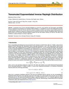
The BIR random variable X is denoted by X ∼ BIR(a, b, θ). The parameters a and b affect the skewness of X by changing the relative tail weights. Figure 1 displays the BIR pdf for several choices of parameter values. Simulating the BIR random variable is relatively simple. Let Y be a random variable distributed according to the usual beta distribution with parameters a and b. Thus, by means of the inverse transformation method, the random variable X given by

√ X=

−

θ log(Y )

follows (3).

2.1

General expansion

Although the cdf and pdf of X require mathematical functions that are widely available in contemporary statistical packages, Eaton et al. (2002) and R Development Core Team (2011) often further analytical and numerical derivations take advantage of power series expansions for the cdf. From the BIR density function (3), the cdf of X can be expressed after usual integration as

Le˜ ao et al.

114

a = b = 2.0

1.0 0.8 0.6

f (x )

0.6 0.0

0.0

0.2

0.2

0.4

0.4

f (x )

0.8

1.2

1.0

1.4

a = b = 0.5

0.5

1.0

1.5

2.0

0.5

2.5

1.0

1.5

(a)

2.5

2.0

2.5

(b)

a = 2.0, b = 0.5

f (x )

0.0

0.0

0.5

0.1

1.0

0.2

1.5

0.3

2.0

0.4

a = 0.5, b = 2.0

f (x )

2.0

x

x

0.5

1.0

1.5

2.0

2.5

0.5

1.0

1.5 x

x

(c)

(d)

Figure 1. Plots of the BIR pdf for θ = 0.5 (solid line), θ = 1.0 (dashed line), θ = 3.0 (dotted line) and θ = 5.0 (bold line).

1 F (x) = B(a, b)

∫

x

0

( ){ ( )}b−1 2θ aθ θ exp − 2 1 − exp − 2 dy. y3 y y

Setting u = θy −2 , it follows that

1 F (x) = B(a, b)

∫

∞ θ x2

exp(−au) {1 − exp(−u)}b−1 du.

(4)

Notice that for |z| < 1 and b > 0 a real non-integer number, we have the power series expansion

Chilean Journal of Statistics

(1 − z)

b−1

∞ ∑ (−1)n Γ(b) n = z , Γ(b − n) n!

115

(5)

n=0

where Γ(·) is the gamma function. Applying this identity into (4) yields ∞

1 ∑ (−1)n Γ(b) F (x) = B(a, b) Γ(b − n)n! n=0

∫

∞

exp{−(a + n)u}du θ x2

and then

{ } ∞ (a + n)θ 1 ∑ (−1)n Γ(b) exp − . F (x) = B(a, b) (a + n) Γ(b − n) n! x2

(6)

n=0

Now, considering the following quantity,

cn (a, b) =

(−1)n Γ(a + b) , (a + n)Γ(a)Γ(b − n)n!

we can write the BIR cdf as a linear combination of IR cdfs. Indeed, we obtain

F (x) =

∞ ∑

cn (a, b) G(x; (a + n)θ).

n=0

In a similar way, the BIR pdf can be expressed according to the following linear combination

f (x) =

∞ ∑

cn (a, b) g(x; (a + n)θ),

n=0

where g(x; (a + n)θ) denotes the IR density function with parameter (a + n)θ. 2.2

Unimodality

The BIR distribution is unimodal for all values of a, b, θ > 0. In order to investigate the critical points of its density function, the first derivative of f (x) with respect to x is given by

( )[ ( )]b−1 d θ2 aθ θ f (x) = exp − 2 1 − exp − 2 dx B(a, b) x6 x x [ ] 6x2 4(b − 1) ( ) , x > 0. × 4a − + θ 1 − exp xθ2

(7)

Le˜ ao et al.

0

2

4

t (y )

6

8

10

116

0.0

0.5

1.0

1.5

2.0

2.5

y

Figure 2. Plots of t(y) for b = 0.25 (solid line), b = 0.5 (dashed line), b = 0.75 (dotted line) and b = 0.95 (bold line).

The signal of this derivative is determined by the expression in the last square brackets, since the remaining terms are all positive. Considering the substitution y = θx−2 , the expression in square brackets becomes

4a −

6 b−1 +4 . y 1 − exp(y)

(8)

Now, we demonstrate that this expression is a monotonic function; therefore, (7) has a single zero, which implies a unique mode. Indeed, the derivative of (8) becomes

t(y) =

6 exp(y) + 4(b − 1) . 2 y [1 − exp(y)]2

For b ≥ 1, this derivative is clearly positive. For 0 < b < 1, Figure 2 displays the numerical results that illustrate the positiveness of the derivative of (8). √ Moreover, let y0 be the zero of (8). The BIR mode location is then given by θ/y0 . Since y0 is independent of θ, the mode location is an increasing function of θ.

3.

Hazard rate function

The survival and hazard rate functions are given by S(x) = 1−F (x) and h(x) = f (x)/S(x), where F (x) and f (x) are the BIR cdf and pdf, respectively. Thus, the hazard rate function of the random variable X is

)]b−1 ( ) [ ( exp − aθ 1 − exp − xθ2 2θ x2 h(x) = . B(a, b) x3 I1−exp(− θ2 ) (b, a) x

Chilean Journal of Statistics

117

Notice that we applied in (2) the symmetry property of the incomplete beta function 1 − Ix (a, b) = I1−x (b, a). We now examine the asymptotic behavior of h(x) when x → ∞ or x → 0. First, we prove that h(x) ∼ 1/x as x → ∞. To establish this result, we verify that limx→∞ h(x)/x−1 is a constant. Indeed, we have

[ ( )]b−1 ( ) exp − aθ h(x) 2θ 1 1 − exp − xθ2 x2 lim = lim x. x→∞ 1/x x→∞ B(a, b) x3 I1−exp(−θ/x2 ) (b, a) ) ( Since exp − aθ x2 → 1 as x → ∞, we can write [ ( )]b−1 2 /x 1 − exp − xθ2 h(x) 2θ lim = lim . x→∞ 1/x B(a, b) x→∞ I1−exp(−θ/x2 ) (b, a) For any value of b > 0, the last expression gives ( rise) to an indeterminate form. Invoking L’Hˆopital’s rule and again considering that exp − aθ x2 → 1 as x → ∞, we obtain

[ ] 1/x2 h(x) ( ) − 2. lim =2θ(b − 1) lim x→∞ 1/x x→∞ 1 − exp − θ2 x Applying the L’Hˆopital rule again we note that the above limit is well-defined and is equal to −2b. Similarly, let us show that h(x) ∼ exp(−aθ/x2 )/x3 as x → 0. In fact, we have immediately that

[ ( )]b−1 1 − exp − xθ2 h(x) 2θ lim lim = x→0 exp(−aθ/x2 )/x3 B(a, b) x→0 I1−exp(−θ/x2 ) (b, a) =

2θ . B(a, b)

Notice also that limx→0 exp(−aθ/x2 )/x3 = 0. Figure 3 displays the behavior of h(x) for selected values of the model parameters.

4.

Moments

The moments play a crucial role in any statistical analysis. The rth moment of X is

2θ E(X ) = B(a, b)

∫

∞

r

(

r−3

x 0

aθ exp − 2 x

)[ ( )]b−1 θ 1 − exp − 2 dx. x

Now, we simplify the above integral. First, letting y = θx−2 , we have

Le˜ ao et al.

118

a = b = 1.0

1.0

h (x )

0.5

2 0

0.0

1

h (x )

3

1.5

4

2.0

a = b = 0.5

0

1

2

3

4

0

5

1

2

3

4

5

4

5

x

x

(a)

(b)

a = 1.5, b = 0.5

0

0.6 0.0

0.2

1

0.4

2

h (x )

h (x )

3

0.8

4

1.0

5

1.2

a = 0.5, b = 1.5

0

1

2

3

4

0

5

1

2

3 x

x

(c)

(d)

Figure 3. Plots of the BIR hazard rate function for θ = 0.5 (solid line), θ = 1.0 (dashed line), θ = 1.5 (dotted line) and θ = 3.0 (bold line).

θr/2 E(X ) = B(a, b)

∫

∞

r

y −r/2 exp(−ay) {1 − exp(−y)}b−1 dy.

0

We refer to the last integral as Sr (a, b). Applying the series expansion (5), for any real r, we obtain

∫

∞

Sr (a, b) =

y −r/2 exp(−ay)

0

=

∞ ∑

∞ ∑

(−1)n

n=0

Γ(b) (−1)n Γ(b − n)n!

n=0

∫

∞

Γ(b) exp(−ny)dy Γ(b − n)n! (9)

y −r/2 exp {−(a + n)y} dy.

0

This integral has a closed-form expression by means of a direct application of the gamma function integral, (Abramowitz and Stegun, 1972). Since a + n > 0, some manipulations

Chilean Journal of Statistics

119

yield

∫

∞

y

−r/2

0

( ) Γ 1 − 2r , exp {−(a + n)y} dy = (a + n)1−r/2

r < 2.

(10)

Therefore, we can rewrite (9) as ∞ ( r)∑ (−1)n Sr (a, b) = Γ(b)Γ 1 − , 2 (a + n)1−r/2 Γ(b − n)n!

r < 2.

n=0

If b > 0 is an integer,we obtain

( ) b ( r)∑ 1 n b−1 Sr (a, b) = Γ 1 − (−1) , 2 n (a + n)1−r/2

r < 2.

n=0

We can write the rth moment of X as

E(X r ) =

θr/2 Sr (a, b), B(a, b)

r < 2.

In particular, for r = 1 and integer an b, we obtain √ ) b ( 1 πθ ∑ b − 1 √ E(X) = . B(a, b) n a+n n=0

Negative moments can also be evaluated. For example, considering r = −1 and for an integer b, we have

√

E(X

−1

( ) b π/θ ∑ 1 n b−1 √ )= (−1) . 2 B(a, b) n (a + n)3 n=0

Notice that attempting to compute (10) outside r < 2 gives undefined forms. For instance, if r = 2, we have

∫

∞ 0

exp[−(a + n)y] dy = E1 (0), y

where E1 (·) is the exponential integral function (Abramowitz and Stegun, 1972), which tends to −∞ as its argument goes to zero. As a consequence, the second moment of X does not exist, as well as all remaining higher order moments. It is known that the second and higher order moments of IR distribution are inexistent (Vod˘a, 1972). As shown above, the BIR distribution inherits this characteristic.

Le˜ ao et al.

120

5.

Quantile function and quantile measures

The quantile function of X is given by

√ Q(u) = F −1 (u) =

−

θ

, log(I−1 u (a, b))

0 < u < 1,

−1 where I−1 u (a, b) is the inverse of the incomplete beta function. The function Iu (a, b) can be written as a power series expansion Wolfram|Alpha (2011)

I−1 u (a, b)

=

∞ ∑

qi [a B(a, b)u]i/a ,

i=1

where q1 = 1 and the remaining coefficients satisfy the following recursion

1 qi = 2 i + (a − 2)i + (1 − a) i−1 ∑ i−r ∑

{ (1 − δi,2 )

i−1 ∑

qr qi+1−r [r(1 − a)(i − r) − r(r − 1)]+

r=2

}

qr qs qi+1−r−s [r(r − a) + s(a + b − 2)(i + 1 − r − s)] ,

r=1 s=1

where δi,2 = 1 if i = 2 and δi,2 = 0 if i ̸= 2. Because the second, third, and fourth moments of the BIR distribution are nonexistent, usual skewness and kurtosis are not defined. However, quantile based measures, such as Bowley skewness (Kenney and Keeping, 1962) and Moors kurtosis (Moors, 1998), can quantify asymmetry and the peakedness of a given distribution. These measures exist even when moments are not available. Bowley skewness and Moors kurtosis are expressed according to

B=

Q(3/4) − 2Q(1/2) + Q(1/4) , Q(3/4) − Q(1/4)

M=

Q(7/8) − Q(5/8) − Q(3/8) + Q(1/8) . Q(6/8) − Q(2/8)

Plots of the Bowley skewness and Moors kurtosis for selected values of a and b are displayed in Figure 4(a). The parameter θ was set to one.

6.

Mean deviations and inequality measures

The amount of scatter in X is measured to some extent by the totality of deviations from the mean (µ) and median (m). These are known as the mean deviation about the mean and the mean deviation about the median given by

Chilean Journal of Statistics

0.14 0.13

0.35

0.12

0.30

0.09

0.10

0.11

Bowley skewness

0.25 0.20

0.07

0.10

0.08

0.15

Bowley skewness

121

0

2

4

6

8

4

10

5

6

7

8

9

10

8

9

10

a

a

(b)

0.3

0.20

0.4

0.25

0.5

Moors kurtosis 0.30

Moors kurtosis 0.6 0.7 0.8

0.35

0.9

1.0

0.40

(a)

0

2

4

6

8

4

10

5

6

7 b

b

(c)

(d)

Figure 4. Plots of the Bowley skewness and Moors kurtosis in terms of (a) a for b = 1.0 (solid curve) and b = 1.5 (dashed curve), b = 3.5 (dotted line) and b = 4.5 (bold line); (b) b for a = 1.0 (solid curve), a = 1.5 (dashed curve), a = 3.5 (dotted line) and a = 4.5 (bold line); (c) a for b = 1.0 (solid curve) and b = 1.5 (dashed curve), b = 3.5 (dotted line) and b = 4.5 (bold line); and (d) b for a = 1.0 (solid curve), a = 1.5 (dashed curve), a = 3.5 (dotted line) and a = 4.5 (bold line).

∫ δ1 (X) = 2µF (µ) − 2µ + 2

∫

∞

xf (x)dx

∞

and δ2 (X) = 2

µ

xf (x)dx − µ,

m

respectively, where µ = E(X) and ∫ z m = Q(1/2). Defining the integral J(z) = 0 xf (x)dx, the measures δ1 (X) and δ2 (X) are given by δ1 (X) = 2µF (µ) − 2J(µ)

and

δ2 (X) = µ − 2J(m),

where F (µ) and F (m) are easily obtained from (2). We now determine J(z). Substituting y = θx−2 in equation (3), we obtain

Le˜ ao et al.

122

∫

z

J(z) = 0

√ ∫ ∞ θ y −1/2 exp(−ay) [1 − exp(−y)]b−1 dy. xf (x)dx = B(a, b) θ/z 2

Considering the power series (5), we have √ ∫ ∞ ∞ θ ∑ (−1)n J(z) = y −1/2 exp{−(a + n)y}dy B(a, b) Γ(b − n)n! θ/z 2 n=0

∞ √ √ √ 1 Γ(b) ∑ (−1)n √ = πθ erfc( θ/z 2 a + n), B(a, b) Γ(b − n)n! a + n n=0

∫∞ 2 where erfc(x) = √2π x e−t dt is the complementary error function. Bonferroni (1930) and Lorenz (1905) curves are inequality measures which have applications in economics, reliability, demography, actuarial sciences, and medicine, among others. They are defined by

1 B(p) = pµ

∫

Q(p) 0

1 J(Q(p)) and xf (x)dx = pµ

1 L(p) = µ

∫

Q(p)

xf (x)dx = 0

1 J(Q(p)), µ

respectively, for 0 < p ≤ 1, see Pundir et al. (2005) for details.

7.

´nyi entropies Shannon and Re

The entropy of a random variable quantifies its associated uncertainty (Song, 2001). Two important entropy measures are the Shannon entropy and its generalization known as the R´enyi entropy. For the BIR distribution, the Shannon entropy is

∫

∞

H(X) = − E{log[f (X)]} = −

( )[ ( )]b−1 } aθ 2θ θ exp − 2 =− f (x) log 1 − exp − 2 dx B(a, b) x3 x x 0 ( ) ∫ ∞ ∫ ∞ 2θ =− log f (x)dx + 3 log(x)f (x)dx B(a, b) 0 0 [ ( )] ∫ ∞ ∫ ∞ 1 θ + aθ f (x)dx − (b − 1) log 1 − exp − 2 f (x)dx, x2 x 0 0 ∫

∞

{

f (x) log[f (x)]dx 0

where the first of the last four integrals is equal to − log[2θ/ B(a, b)]. The second integral can be calculated as follows

Chilean Journal of Statistics

∫ 0

∞

123

{

( )[ ( )]b−1 } 2θ aθ θ log(x)f (x)dx = log(x) exp − 2 1 − exp − 2 dx B(a, b) x3 x x 0 { } ∫ ∞ 2θ ∑ (−1)n Γ(b) ∞ log(x) −(a + n)θ = exp dx B(a, b) Γ(b − n)n! 0 x3 x2 ∫

∞

n=0 ∞

=

2θ ∑ (−1)n Γ(b) log[(a + n)θ] + γ , B(a, b) Γ(b − n)n! 4(a + n)θ n=0

where γ is the Euler-Mascheroni constant. The third integral can be expressed by

∫

∞ 0

( )[ ( )]b−1 2θ aθ θ exp − 2 1 − exp − 2 dx B(a, b) x5 x x 0 ( ) ∞ } { ∫ ∞ 2θ 1 aθ ∑ (−1)n Γ(b) −nθ = exp − 2 exp dx B(a, b) 0 x5 x Γ(b − n)n! x2 n=0 { } ∫ ∞ 2θ ∑ (−1)n Γ(b) ∞ 1 −(a + n)θ = exp dx. B(a, b) Γ(b − n)n! 0 x5 x2

1 f (x)dx = x2

∫

∞

n=0

Setting t =

(a+n)θ x2 ,

∫

we obtain

∞ 0

∞

1 2θ ∑ (−1)n Γ(b) f (x)dx = x2 B(a, b) Γ(b − n)n! n=0

=

1 θ B(a, b)

∞ ∑ n=0

∫ 0

∞

exp(−t) dt [2(a + n)θ]2

(−1)n Γ(b) 1 . Γ(b − n)n! (a + n)2

Considering the fourth integral, let u = θx−2 . From the power series expansion log(1 + z) = z + 12 z 2 − 13 z 3 − · · · , we can write

∫

∞

log[1 − exp(−θ/x2 )]f (x)dx =

0

1 B(a, b)

=−

∫

∞

0

1 B(a, b)

1 = B(a, b)

∫

∞ ∞∑ 0

∞ ∞ ∑ ∑ k=1 n=0 ∞

=

log{1 − exp(−u)} exp(−au)[1 − exp(−u)]b−1 du

∞

(−1)n+1 Γ(b) kΓ(b − n) n!

∫

∞

exp {−u(a + k + n)} du

0

1 ∑∑ (−1)n+1 Γ(b) . B(a, b) k(a + k + n)Γ(b − n) n! k=1 n=0

Finally, we obtain

k=1

exp{−u(k + a)} [1 − exp(−u)]b−1 du k

Le˜ ao et al.

124

{ H(X) = − log

2θ B(a, b)

} +

[ ] ∞ ∞ ∑ Γ(b) ∑ (−1)n a 3 log{(a + n)θ} + γ 1 + + (b − 1) . B(a, b) Γ(b − n) n! 2 a+n (a + n)2 k(a + k + n) n=0

k=1

Now, the R´enyi entropy can be expressed as 1 Hα (X) = log 1−α

(∫

)

∞

α > 0, α ̸= 1,

α

f (x) dx ,

(11)

0

where α > 0 and α ̸= 1. Notice that when α → 1, the R´enyi entropy converges to the Shannon entropy. For calculating (11), we apply (3) and consider the power series expansion (5) yielding

∫

∞ 0

[

]α ∞ ∑ 2θ (−1)n f (x) dx = Γ(α(b − 1) + 1) B(a, b) Γ(α(b − 1) + 1 − n) n! n=0 { } ∫ ∞ θ −3α × x exp −(aα + n) 2 dx. x 0 α

The last integral can be evaluated as follows. Let u = θx−2 . Then, we have

∫

∞

−3α

x 0

{

θ exp −(aα + n) 2 x

}

∫

∞

dx =

u

3(α−1) 2

0

( =

1 aα + n

exp {−(aα + j)u} du

) 3α−1

(

2

Γ

3α − 1 2

) .

Finally, we obtain

∫

∞ 0

[

2θ f (x)α dx = B(a, b)

]α

Γ 2θ

8.

( 3α−1 ) 2 3(α−1) 2

+1

∞ ∑ n=0

(−1)n (aα + n)

3α−1 2

Γ(α(b − 1) + 1) . Γ(α(b − 1) + 1 − n)n!

Order statistics

Here, we present an explicit expression for the density function fi:n (x) of the ith order statistic Xi:n in a random sample of size n from the BIR distribution. Consider the wellknown result

fi:n (x) = for i = 1, . . . , n.

f (x) F (x)i−1 {1 − F (x)}n−i , B(i, n − i + 1)

Chilean Journal of Statistics

125

Applying the binomial expansion in the above equation, we obtain

) n−i ( ∑ f (x) n−i fi:n (x) = (−1)l F (x)i+l−1 . B(i, n − i + 1) l l=0

Inserting (3) and (6) in the last equation, fi:n (x) can be expressed as

( )[ ( )]b−1 ∑ ) n−i ( aθ θ n−i 2θ (−1)l exp − 1 − exp − fi:n (x) = B(i, n − i + 1)x3 x2 x2 l B(a, b)i+l  ×

( ) Γ(b) (a + j)θ  exp − a + j Γ(b − j)j! x2

∞ ∑ (−1)j j=0

l=0

i+l−1

(12) ,

for b > 0 real non-integer. Now, using the following identity

(

∞ ∑

)k ai

=

∞ ∑

···

m1 =0

i=0

∞ ∑

am1 · · · amk ,

mk =0

for k positive integer, we can write (12) as

fi:n (x) =

n−i ∑ ∞ ∑ l=0 m1 =0

···

∞ ∑

δi,l fi,l (x),

(13)

mi+l−1 =0

where

{ } )[ ( θ )]b−1 ( θ ∑i+l−1 2θ exp − aθ 1 − exp − exp − (a + m ) j j=1 x2 x2 x2 ( ) fi,l (x) = , ∑ i+l−1 x3 B a(i + l) + j=1 mj , b and

) ( ) ∑i+l−1 mj , b Γ(b)i+l−1 B a(i + l) + j=1 . ∏ B(a, b)i+l B(i, n − i + 1) i+l−1 j=1 (a + mj )Γ(b − mj )mj !

(−1)l+ δi,l =

∑i+l−1 j=1

(

mj n−i l

∑i+l−1 , b, θ) distribution. Note that fi,l (x) is the density function of the BIR(a(i + l) + j=1 Also, the constants δi,l are obtained given i, n, l and a sequence of indices m1 , . . . , mi+l−1 . The sums in (13) extend over all (i + l)-tuples (l, m1 , . . . , mi+l−1 ) of non-negative integers. These sums indicate that the density function of the BIR order statistics is a linear combination of BIR densities. So, several structural quantities of the BIR order statistics can be obtained from those of BIR distribution.

Le˜ ao et al.

126

9.

Maximum likelihood estimation and information matrix

Consider independent BIR distributed random variables X1 , . . . , Xn with parameter vector λ = (a, b, θ)T . The log-likelihood function ℓ(λ) for the BIR model reduces to

n ∑

n ∑ 1 ℓ(a, b, θ) =n[log(2θ) − log{B(a, b)}] − 3 log(xi ) − aθ x2 i=1 i=1 i { ( )} n ∑ θ + (b − 1) log 1 − exp − 2 . xi i=1

The elements of the score vector are:

∑ 1 ∂ ℓ(a, b, θ) = n[ψ(a + b) − ψ(a)] − θ , ∂a x2i n

Ua (λ) =

i=1

)} θ , log 1 − exp − 2 x i i=1 ) ( θ n n exp − ∑ ∑ 2 x ∂ n a [ (i )] , Uθ (λ) = ℓ(a, b, θ) = − + (b − 1) 2 ∂θ θ 2 1 − exp − θ x i x i=1 i=1 i x2 ∂ Ub (λ) = ℓ(a, b, θ) = n[ψ(a + b) − ψ(b)] + ∂b

n ∑

{

(

i

where ψ(·) is the digamma function, see Abramowitz and Stegun (1972). The ML equations can be solved numerically for a, b, and θ. Under standard regularity conditions (Cox and Hinkley, 1974) that are fulfilled for the proposed model whenever the parameters are in the interior of the parameter space, the observed information matrix I(λ) can be employed for interval estimation of the model parameters and for hypothesis tests. The BIR observed information matrix is given by



 Uaa (λ) Uab (λ) Uaθ (λ) I(λ) = −  Uab (λ) Ubb (λ) Ubθ (λ)  , Uaθ (λ) Ubθ (λ) Uθθ (λ)

whose elements are

Chilean Journal of Statistics

127

∂ Ua (λ) =n [ψ1 (a + b) − ψ1 (a)] , ∂a ∂ Uab (λ) = Ua (λ) =nψ1 (a + b), ∂b n ∑ ∂ 1 Uaθ (λ) = Ua (λ) = − 2, ∂θ x i=1 i

Uaa (λ) =

∂ Ub (λ) =n [ψ1 (a + b) − ψ1 (b)] , ∂b ) ( θ n exp − ∑ x2 ∂ )] , [ (i Ubθ (λ) = Ub (λ) = ∂θ 2 1 − exp − θ x 2 i=1 i xi ( )[ ( )] θ n exp − θ2 2 − exp − ∑ 2 xi xi ∂ n Uθθ (λ) = Uθ (λ) = − 2 − (b − 1) , )]2 [ ( ∂θ θ i=1 x4i 1 − exp − xθ2 Ubb (λ) =

i

d and ψ1 (·) is the polygamma function, which satisfies ψ1 (x) = dx ψ(x). Since the Fisher information matrix is not available, the standard errors (SEs) are obtained by square-rooting the diagonal elements of the covariance matrix, i.e., the inverse of the second derivative matrix of the log-likelihood function, evaluated at the ML estimates (MLEs). We can compute the maximum values of the unrestricted and restricted log-likelihoods to obtain the likelihood ratio (LR) statistics for testing some sub-models of the BIR distribution. The (0) LR statistic for testing the null hypothesis H0 : λ1 = λ1 versus the alternative hypothesis (0) ˆ − ℓ(λ)}, ˜ ˆ and λ ˜ are the MLEs under the H1 : λ1 ̸= λ1 is given by w = 2{ℓ(λ) where λ alternative and null hypotheses, respectively. The statistic w is asymptotically distributed as χ2k , where k is the dimension of the subset λ1 of interest.

10.

Application to real data

In this section, the BIR is fitted to an example of real data concerning the tensile strength, which were originally reported by Bader and Priest (1982) and can also be found in Ghitany et al. (2011). These data represent the strength measured in GPa for single carbon fibers and impregnated 1000-carbon fiber tows. Table 1 provides some descriptive measures for strength data, which include central tendency statistics, the standard deviation (SD), and coefficients of variation (CV), of skewness (CS) and of kurtosis (CK), among others. These data are fitted by using the BIR, exponentiated inverse Rayleigh (EIR) (Gupta et al., 1998) and IR distributions. All these distributions are common models for lifetime data. The ML estimators of the model parameters are obtained by using the Broyden-FletcherGoldfarb-Shanno (BFGS) quasi-Newton nonlinear optimization algorithm with analytic derivatives; for more details, see Nocedal and Wright (1999) and Mittelhammer et al. (2000, p. 199). Computational implementation was performed in Ox matrix programming language (Doornik, 2006). Tables 2 report the MLEs of the model parameters (SEs in parentheses) for each model. It is also shown the values for the Akaike information criterion (AIC) (Akaike, 1973),

Le˜ ao et al.

128 Table 1. summary statistics.

n 69

Min. 1.312

Median 2.478

Mean 2.451

2.0

2.5

3.0

Max. 3.585

SD 0.495

CV 20.19%

CS −0.028

CK −0.144

0.6 0.4

Density

3.0 2.5 1.0

0.0

1.5

0.2

2.0

empirical quantiles

3.5

0.8

4.0

Data set strength

1.5

1.0

1.5

2.0

(a)

2.5

3.0

3.5

4.0

x

theoretical quantiles

(b)

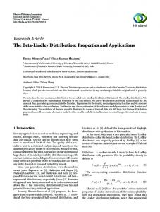
Figure 5. (a) QQ plot with envelope for the BIR distribution and (b) fitted densities of the BIR (bold line), EIR (dashed line) and Inverse Rayleigh (dotted line) distributions for strength data.

Bayesian information criterion (BIC) (Schwarz, 1978), bias-corrected Akaike information criterion (BAIC) (Hurvich and Tsai, 1989), Hannan-Quinn information criterion (HQIC) (Hannan and Quinn, 1979), and Kolmogorov-Smirnov (KS) goodness-of-fit test. The KS test indicates that there is not sufficient statistical evidence as for supporting that the data do not follow the BIR and EIR distributions; see Table 2. In Figure 5(a), we present the quantile against quantile (QQ) plot with envelope, which allows us to compare the empirical distribution of the data for the BIR distribution. This graphical goodness-of-fit method supports the result obtained by the KS test. In terms of AIC, BAIC, and HQIC values, the horse race winner is the BIR distribution; see Table 2. Plots of the estimated densities of the BIR, EIR and IR models fitted to these data are displayed in Figure 5(b). The overall results suggest that the BIR distribution is superior to the remaining distributions in terms of model fitting. Table 2. Parameter estimates, goodness-of-fit measures and KS statistics for strength data.

Estimates (SEs) bb b a BIR 0.2686 69.3250 (0.0394) (21.6710) EIR − 10.2986 (−) (8.8910) IR − − (−) (−)

θb 42.5446 (2.1419) 15.6410 (1.5547) 5.2111 (0.6273)

Goodness-of-fit measures AIC BIC BAIC HQIC 104.77 111.47 174.14 107.43

KS statistics

p-value

0.0519

0.9923

108.14 112.61 177.32 109.91

0.0777

0.7985

178.83 181.06 247.89 179.71

0.3549

< 0.0001

In order to confirm that the log-likelihood function is well behaved and that an unequivocal optimum has been reached, we plot the profiles of the negative log-likelihood function

0.1

0.2

0.3

0.4

0.5

negative log−likelihood 68.0

68.5

^a

69.0

69.5 b^

70.0

70.5

71.0

49.40 49.45 49.50 49.55 49.60 49.65 49.70

49.388 49.387 49.384

50

49.385

49.386

negative log−likelihood

70 65 60 55

negative log−likelihood

129

49.389

75

Chilean Journal of Statistics

41.0

(b) b b

(a) b a

41.5

42.0

42.5 θ^

43.0

43.5

44.0

(c) θb

Figure 6. Profiles of the negative log-likelihood function for the BIR distribution.

for the BIR distribution; see Figure 6. Note that in each case the parameter estimate had a nice quadratic neighborhood. Here, we test the null hypothesis H0 : EIR against the alternative hypothesis H1 : BIR and also H0 : IR against H1 : BIR, i.e., H0 : a = 1 against H1 : b ̸= 1 and H0 : a = b = 1 against H1 : H0 is false, respectively. The LR statistics are listed in Table 3. For any usual significance level, we reject both null models (EIR and IR) in favor of the alternative BIR model. Table 3. LR tests.

Models BIR vs EIR BIR vs IR

Hypotheses H0 : a = 1 vs H1 : H0 is false H0 : a = b = 1 vs H1 : H0 is false

11.

w 5.370 78.06

p-valor 0.0205 < 0.0001

Conclusion

In this work, we study the beta inverse Rayleigh distribution as a generalization of the inverse Rayleigh distribution. We also provide a better foundation for some mathematical properties for this distribution, including the derivation of the hazard rate function, moments, quantile measures, mean deviations, entropy measures and order statistics. The model parameters are estimated by maximum likelihood. An application of the BIR distribution to a real data set indicates that this distribution outperforms both the exponentiated inverse Rayleigh and inverse Rayleigh distributions.

Acknowledgements The authors acknowledge support from CAPES, CNPq, and FACEPE. We are also grateful to the editor and two anonymous referees for helpful comments and suggestions.

References Abramowitz, M., Stegun, I.A. (eds), 1972. Handbook of Mathematical Functions with Formulas, Graphs, and Mathematical Tables, Dover Publications, New York.

130

Le˜ ao et al.

Akaike, H., 1973. Information Theory and an Extension of the Maximum Likelihood Principle in B. N. Petrov and F. Csaki (eds), Proceedings of the Second International Symposium on Information Theory, 1, Akademiai Kiado, pp. 267-281. Akinsete, A., Famoye, F., Lee, C., 2008. The beta-Pareto distribution. Statistics, 42, 547563. Amoroso, L., 1925. Ricerche intorno alla curva dei redditi. Annali de Mathematica, 2, 123-159. Barreto-Souza, W., Santos, A.H.S. and Cordeiro, G.M., 2010. The beta generalized exponential distributions. Journal of Statistical Computation and Simulation, 80, 159-172. Barreto-Souza, W., Cordeiro, G.M., Simas, A.B., 2011. Some results for beta Fr´echet distribution. Communications in Statistics - Theory and Methods, 40, 789-811. Bonferroni, C., 1930. Elementi di Statistica Generale, Seeber - Firenze. Bader, M. G., Priest, A.M., 1982. Statistical aspects of fiber and bundle strength in hybrid composites, in Progress in Science and Engineering Composites, Proceedings of the 4th International Conference on Composite Materials (ICCM-IV), Japan Society for Composite Materials, Tokyo, T. Hayashi, K. Kawata, and S. Umekawa, eds., ICCM, Tokyo, pp. 1129-1136. Cintra, R.J., Rˆego, L.C., Cordeiro, G.M., Nascimento, A.D.C., 2011. Beta Generalized Normal Distribution with an Application for SAR Image Processing. Accepted. Cox, D.R.. Hinkley, D.V., 1974. Theoretical Statistics. Chapman and Hall, London Doornik, J.A., 2006. An Object-Oriented Matrix Language, 5 edn, Timberlake Consultants Press, London, UK. Eaton, J.W., Bateman, D., Hauberg, S., 2002. GNU Octave Manual Version 3, Network Theory Limited. Eugene, N., Lee, C., Famoye, F., 2002. Beta-normal distribution and its applications. Communications in Statistics - Theory and Methods, 32, 497-512. Gharraph, M., 1993. Comparison of estimators of location measures of an inverse Rayleigh distribution. The Egyptian Statistical Journal, 37, 295-309. Ghitany, M.E., Al-Jarallah, R.A., Balakrishnan, N., 2011. On the existence and uniqueness of the MLEs of the parameters of a general class of exponentiated distributions. Statistics, 47, 37-41. Good, I.J., 1953. The population frequencies of the species and the estimation of population parameters. Biometrika, 40, 237-260. Gupta, A.K., Nadarajah, S., 2004. On the moments of the beta normal distribution. Communications in Statistics - Theory and Methods, 33, 1-13. Gupta, R.C., Gupta, P.L., Gupta, R.D., 1998. Modeling failure time data by Lehman alternatives. Communications in Statistics - Theory and Methods, 27, 887-904. Hannan, E.J., Quinn, B.G., 1979. The determination of the order of an autoregression. Journal of the Royal Statistical Society, B, 41, 190-195. Hoskings, J.R.M., Wallis, J.R., 1987. Parameter and quantile estimation for the generalized Pareto distribution. Technometrics, 29, 339-349. Hurvich, C.M., Tsai, C.L., 1989. Regression and time series model selection in small samples. Biometrika, 76, 297-307. Iliescu, D.V., Vod˘a, V.Gh., 1973. Studiul variabilei aleatoare repartizate invers Rayleigh. Studii ¸si Cerc. Mat. Bucure¸sti, 25, 1507-1521. Kenney, J.F., Keeping, E.S., 1962. Mathematics of Statistics, Vol. Part 1, 3 edn, Princento, New Jersey. Lee, C., Famoye, F., Olumolade, O., 2007. Beta-Weibull distribution: some properties and applications to censored data. Journal of Modern Applied Statistical Methods, 6, 173-186. Lorenz, M., 1905. Methods of measuring the concentration of wealth. Publications of the

Chilean Journal of Statistics

131

American Statistical Association, 9, 209-219. McDonald, J.B., 1984. Some generalized functions for the size distribution of income. Econometrica, 52, 647-663. Mittelhammer, R.C., Judge, G.G., Miller, D.J., 2000. Econometric Foundations. Cambridge University Press, New York. Mohsin, M., Shahbaz, M.Q., 2005. Comparison of Negative Moment Estimator with Maximum Likelihood Estimator of Inverse Rayleigh Distribution. Pakistan Journal of Statistics and Operation Research, 1, 45-48. Moors, J.J.A., 1998. A quantile alternative for kurtosis. Journal of the Royal Statistical Society D, 37, 25-32. Nadarajah, S., Gupta, A.K., 2004. The beta Frechet distribution. Far East Journal of Theoretical Statistics, 15, 15-24. Nadarajah, S., Kotz, S., 2004. The beta Gumbel distribution. Mathematical Problemas in Engineering, 10, 323-332. Nadarajah, S., Kotz, S., 2005. The beta exponential distribution. Reliability Engineering and System Safety, 91, 689-697. Nocedal, J., Wright, S.J., 1999. Numerical Optimization. Springer. Pescim, R.R., Dem´etrio, C.G.B., Cordeiro, G.M., Ortega, E.M.M., Urbano, M.R. (2010). The beta generalized half-normal distribution. Computational Statistics and Data Analysis, 54, 945-957. Pundir, S., Arora, S., Jain, K., 2005. Bonferroni Curve and the related statistical inference. Statistics & Probability Letters, 75, 140-150. R Development Core Team, 2011. R: A Language and Environment for Statistical Computing, R Foundation for Statistical Computing, Vienna, Austria, http://www.r-project. org. Rˆego, L.C., Cintra, R.J., Cordeiro, G.M., 2012. On some properties of the beta normal distribution. Communications in Statistics - Theory and Methods, 41, 3722-3738. Rosaiah, K., Kantam, R.R.L., 2005. Acceptance Sampling Based on the Inverse Rayleigh Distribution. Economic Quality Control, 20, 277-286. Schwarz, G., 1978. Estimating the Dimension of a Model. Annals of Statistics, 6, 461-464. Soliman, A., Amin, E., Abd-El Aziz, A., 2010. Estimation and Prediction from Inverse Rayleigh Distribution Based on Lower Record Values. Applied Mathematical Sciences, 4(62), 3057-3066. Song, K.S., 2001. R´enyi information, loglikehood and an intrinsic distribution measure. Journal of Statistical Planning and Inference, 93, 51-69. Tre$ ier, V.N., 1964. Doklady Akad. Nauk, Belorus SSR. Vod˘a, V. Gh, 1972. On the inverse Rayleigh distributed random variable. Rep. Stat. Appl. Res. JUSE, 19(4), 13-21. Wolfram|Alpha, 2011. Inverse of the regularized incomplete beta function, http:// functions.wolfram.com/06.23.06.0001.01.