A New Node-to-Node Approach to A New Node to ... - IDEALS @ Illinois

NSEL Report Series Report No. NSEL-009 May 2008

A New Node Node-to-Node to Node Approach to Contact/Impact Problems for Two-Dimensional Elastic Solids Subject to Finite Deformation

Daqing Xu and Keith D. Hjelmstad

NEWMARK STRUCTURAL ENGINEERING LABORATORY

Department of Civil and Environmental Engineering University of Illinois at Urbana-Champaign

UILU-ENG-2008-1803

ISSN: 1940-9826

© The Newmark Structural Engineering Laboratory

The Newmark Structural Engineering Laboratory (NSEL) of the Department of Civil and Environmental Engineering at the University of Illinois at Urbana-Champaign has a long history of excellence in research and education that has contributed greatly to the state-of-the-art in civil engineering. Completed in 1967 and extended in 1971, the structural testing area of the laboratory has a versatile strong-floor/wall and a three-story clear height that can be used to carry out a wide range of tests of building materials, models, and structural systems. The laboratory is named for Dr. Nathan M. Newmark, an internationally known educator and engineer, who was the Head of the Department of Civil Engineering at the University of Illinois [1956-73] and the Chair of the Digital Computing Laboratory [1947-57]. He developed simple, yet powerful and widely used, methods for analyzing complex structures and assemblages subjected to a variety of static, dynamic, blast, and earthquake loadings. Dr. Newmark received numerous honors and awards for his achievements, including the prestigious National Medal of Science awarded in 1968 by President Lyndon B. Johnson. He was also one of the founding members of the National Academy of Engineering.

Contact: Prof. B.F. Spencer, Jr. Director, Newmark Structural Engineering Laboratory 2213 NCEL, MC-250 205 North Mathews Ave. Urbana, IL 61801 Telephone (217) 333-8630 E-mail: [email protected]

This technical report is based on the first author's doctoral dissertation under the same title which was completed in April 2008. The second author served as the dissertation advisor for this work. The cover photographs are used with permission. The Trans-Alaska Pipeline photograph was provided by Terra Galleria Photography (http://www.terragalleria.com/).

Abstract Contact analysis is an important branch of solid mechanics. Numerical simulation using the finite element method has become the dominant approach recently because of the high nonlinearity of contact problems. In the traditional Lagrangian description for solid mechanics, the numerical nodes are attached to the material particles, making it impossible to maintain node-to-node contact due to independent deformation. Various node-to-segment or segment-to-segment treatments are proposed to discretize the contact interface. But some issues still exist. Specifically, mesh distortion or element entanglement may be present if deformation is large. A new node-to-node approach for 2D contact/impact problems subject to finite deformation is proposed in this report to offer an alternative approach to these traditional methods, wherein node-to-node contact is maintained throughout the contact process. This method is based on the Arbitrary Lagrangian-Eulerian algorithm (ALE). One or both bodies in the two-body contact problem have an ALE mesh, which is independent of the material particles and has prescribed motion set to maintain node-to-node contact. The strategy of the ALE mesh motion has two steps: (1) to move nodes in the active set to maintain node-to-node contact (2) to smooth ALE mesh to improve mesh quality using the Laplacian or angle-based smoothing algorithm. Problems of interest in this study are contact/impact problems wherein the implicit mid-point rule is used as the primary time stepping algorithm to find the solution incrementally. In order to conserve the system energy, the persistency condition is incorporated as the contact constraint. The augmented Lagrangian method is primarily used to apply contact constraints. Non-classical Coulomb friction laws are used where friction is present. Several quasi-static and impact examples are given to demonstrate the performance and validity of the new approach.

Table of Contents 1

Introduction . . . . . . . . . 1.1 Background information 1.2 Motivation . . . . . . . . 1.3 Outline of the report . . .

. . . .

. . . .

. . . .

. . . .

. . . .

. . . .

. . . .

. . . .

. . . .

. . . .

. . . .

. . . .

. . . .

. . . .

. . . .

. . . .

. . . .

. . . .

. . . .

. . . .

. . . .

. . . .

. . . .

. . . .

. . . .

. . . .

1 1 6 8

2 Background information of contact/impact problems . 2.1 Definition and notation of contact problems . . . . 2.1.1 Gap function and local coordinate system . 2.1.2 Definition of contact tractions . . . . . . . 2.1.3 Consideration of friction . . . . . . . . . . 2.1.4 Contact detection . . . . . . . . . . . . . . 2.2 Treatment of contact constraints . . . . . . . . . . 2.2.1 Classical Lagrange multiplier . . . . . . . 2.2.2 Penalty method . . . . . . . . . . . . . . . 2.2.3 Augmented Lagrangian method . . . . . . 2.3 Problem description in strong and weak form . . . 2.3.1 Strong form . . . . . . . . . . . . . . . . . 2.3.2 Weak form . . . . . . . . . . . . . . . . . 2.4 Definition and notation of ALE formulation . . . . 2.4.1 Definition of kinetic variables . . . . . . . 2.4.2 Convective velocity . . . . . . . . . . . . . 2.4.3 Virtual work equation in ALE description .

. . . . . . . . . . . . . . . . .

. . . . . . . . . . . . . . . . .

. . . . . . . . . . . . . . . . .

. . . . . . . . . . . . . . . . .

. . . . . . . . . . . . . . . . .

. . . . . . . . . . . . . . . . .

. . . . . . . . . . . . . . . . .

. . . . . . . . . . . . . . . . .

. . . . . . . . . . . . . . . . .

. . . . . . . . . . . . . . . . .

. . . . . . . . . . . . . . . . .

. . . . . . . . . . . . . . . . .

9 9 9 12 13 14 15 15 16 16 18 18 20 21 21 23 24

3 Time-stepping algorithm and energy conservation . . 3.1 Mid-point rule . . . . . . . . . . . . . . . . . . . . 3.2 Persistency condition . . . . . . . . . . . . . . . . 3.3 Conservation of total energy . . . . . . . . . . . . 3.3.1 Energy conservation in frictionless contact 3.3.2 Energy conservation in frictional contact .

. . . . . .

. . . . . .

. . . . . .

. . . . . .

. . . . . .

. . . . . .

. . . . . .

. . . . . .

. . . . . .

. . . . . .

. . . . . .

. . . . . .

26 27 28 31 32 33

4 Mesh motion strategy . . . . . . . . . . . . . . . . . . . . 4.1 Mesh motion strategy in node-to-node contact . . . . . 4.1.1 Surface mesh motion . . . . . . . . . . . . . . 4.1.2 Mesh smoothing algorithms in two dimensions 4.2 Example of mesh motion . . . . . . . . . . . . . . . . 4.3 Interpolation of kinetic variables . . . . . . . . . . . .

. . . . . .

. . . . . .

. . . . . .

. . . . . .

. . . . . .

. . . . . .

. . . . . .

. . . . . .

. . . . . .

. . . . . .

35 36 36 40 44 46

5 Finite element implementation . . . . . . . . . . . . . . . . . . . 5.1 Spatial discretization . . . . . . . . . . . . . . . . . . . . . . 5.1.1 Four nodes isoparametric element Q4 . . . . . . . . . 5.1.2 Discretization on contact interface . . . . . . . . . . . 5.1.3 Spatial discretization . . . . . . . . . . . . . . . . . . 5.2 Temporal discretization . . . . . . . . . . . . . . . . . . . . . 5.3 Linearization of governing equation . . . . . . . . . . . . . . 5.4 Solution process . . . . . . . . . . . . . . . . . . . . . . . . . 5.5 Implementation of alternative approach to energy conservation

. . . . . . . . .

. . . . . . . . .

. . . . . . . . .

. . . . . . . . .

. . . . . . . . .

. . . . . . . . .

48 49 49 50 52 55 55 57 59

6 Numerical examples . . . . . . . . . . . . . . . . . . . . . 6.1 Frictional elastic contact with finite sliding . . . . . . . 6.2 Quasi-static Hertzian contact problem . . . . . . . . . 6.3 Frictional contact of delamination analysis . . . . . . . 6.4 Frictionless impact of a ring against an obstacle . . . . 6.5 Frictional impact of blocks with fast sliding . . . . . . 6.6 Frictional impact of blocks with tilted contact interface

. . . . . . .

. . . . . . .

. . . . . . .

. . . . . . .

. . . . . . .

. . . . . . .

61 62 65 70 75 82 93

. . . . . . .

. . . . . . .

. . . . . . .

. . . . . . .

7 Conclusions and future work . . . . . . . . . . . . . . . . . . . . . . . . . . 104 7.1 Conclusions . . . . . . . . . . . . . . . . . . . . . . . . . . . . . . . . . 104 7.2 Future work . . . . . . . . . . . . . . . . . . . . . . . . . . . . . . . . . 104 References . . . . . . . . . . . . . . . . . . . . . . . . . . . . . . . . . . . . . . 106

Chapter 1

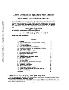
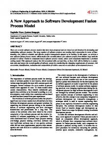
Introduction 1.1 Background information Contact is a common phenomenon in mechanical, civil and astronautical engineering when two solid objects try to occupy the same position. Material nonlinearity, geometric nonlinearity and transient effects are often involved in the mechanical process and must be considered in the analysis. Two typical examples are shown here. Figure1.1 shows the forging process of a steel plate. The right two dies are used as fixed supports and the middle one punches downward slowly to stretch the plate to the expected shape. The plate endures large deformation and partly enters the plastic range of response. In this example, contact interfaces are the common surfaces shared by the plate and the dies. The forging process may be treated as quasi-static because deformation changes slowly. Figure1.2 shows an impact test of an automobile where the car crashes into a rigid obstacle to evaluate its safety. The contact interfaces here comprise part of the bumper, hood and some internal instruments in succession. After impact, the car’s hood and body become folded and the bumper is broken due to violent impact forces. The contact process in this example is so fast that transient effects must be considered.

Fig. 1.1: Steel plate in forming process, from manual of ABAQUS6.3

1

Fig. 1.2: Crash test of an automobile, from www.safercar.gov

From the two examples, it is evident that contact bodies cannot penetrate into each other. That is one of the most important property for contact problems. One may also observe that the motion of the contact bodies is not necessarily smooth, especially on the contact interface. The displacement and velocity fields can jump when contact occurs. Besides these observations, one may note that the exact contact interface is unknown a priori and cannot be treated as the Dirichlet or Neumann boundary because both tractions and displacements are unknown. Although contact problems share the same fundamental laws of solid mechanics, e.g., momentum balance and mass conservation laws as other problems, they fall into the most difficult category of problems in solid mechanics and involve more conceptual, mathematical and computational efforts. Other contact examples like wear and lubrication in mechanical engineering, mechanical impact in astronautical engineering and drilling in geological investigation are also common. In the last several decades, investigation of contact has become an important branch of solid mechanics. The first success in solving a contact problem was accomplished by Hertz [27]. He studied the contact problem of two spherical elastic bodies and gave a formulation of the pressure distribution and indentation in the contact interface. After that, the important advance in contact theory was achieved by Fichera [19] where he first treated the contact problem as a variational inequality. Another milestone was marked by Kikuchi and Oden [39] wherein they investigated series of contact problems theoretically and numerically. Although other progress was made after the 1970s, theoretical advance has been seriously hindered by the inherent complexity of the problem. Recent progress has been obtained from numerical simulations where the finite element method is used. The early efforts of numerical simulations are focused on frictionless contact problems with small 2

elastic deformations. Conry and Seireg [14] applied a simplex-type algorithm to Hertzian type problems and beams contact problems under the elastic assumption. Francavilla and Zienkiewicz [21] focused on construction of the tangent matrix and treated the contact pressure as quasi-linear for some frictionless contact problems. Hughes and Taylor [37] studied some contact/impact problems and discussed different topics like spatial and temporal discretization, contact bodies in different dimensions and contact release conditions. Since the finite element method employs the discretized configurations instead of the really continuous one, the contact pairs, that are isolated nodes in the contact interface, were assumed to be in node-to-node contact status initially in the early proposed approaches. The assumption of an infinitesimal deformation makes it possible to omit mismatching of the contact pair in the deformed configurations. Another character of the early efforts is that the Signorini’s problem (contact between a flexible body and a rigid obstacle) drew much attention because researchers needed not to worry about unmatched meshes. For contact problems involving two flexible bodies, the node-to-node contact assumption is a big encumbrance. Various approaches were proposed to treat the mismatched contact pairs as known as the node-to-segment (one pass), the node-to-segment (two pass), the intermediate contact surface, and the segment-to-segment approach. These methods are well known now as the unilateral contact law to treat the impenetrability in the contact interface. The one pass node-to-segment approach [5] distinguishes a “master body” from a “slave body” and the slave body is prohibited from penetrating into the master body. This method fails to pass the patch test because it is unable to transfer contact pressures accurately through the mismatched contact nodes. The two-pass node-to-segment approach [62] [33] searches the contact interface twice and uses the ordinary and reversed definition of the master and slave bodies. This approach passes the patch test for linear elements, but the main drawback is that the overconstrained definition impairs the stability performance. The intermediate surface approach introduced a contact element defined by the nodes in the contact interface and their projections [61] [16]. The behavior of the method in [61], where 2D linear elements are used, is similar to the two-pass node-to-segment approach in that it is still overconstrained but passes the patch test. The algorithm in [16], where 2D quadratic elements are used, removes the redundant constraints and passes the patch test with the sacrifice of losing stability to some degree [18]. The segment-tosegment approach [18] [51] [70] were proposed recently to try to overcome the weakness of previous approaches. The mortar method, initially developed to remedy dissimilarly meshed configurations, is reported to have good convergence performance in tied contact problems [70]. All these approaches are constructed on the Lagrangian description and there is a common assumption that node-to-node contact status cannot be maintained for the Lagrangian mesh.

Current applications of the finite element method to problems in solid mechanics are mostly based on the Lagrangian description. The material particles are attached to 3

the numerical mesh and there is no convective velocity between mesh nodes and material particles. One benefit of the Lagrangian description is that the governing equation is simple due to the absence of convective velocity. Another benefit is that material motion and stress-strain status are conveniently and accurately computed from the mesh motion. Whenever the mesh motion is determined, the kinematic fields of material particles are also obtained. The quadrature points always coincide with the same material particles that numerical simulation of path-dependent material, like elastic-plastic material, is greatly simplified. However, the coincidence between the mesh and the material particles in the Lagrangian description may cause mesh distortion and element entanglement when deformation is large, e.g., in the metal forming simulations. Solution accuracy and convergence are seriously impaired by the defective mesh. In the fluid mechanics field, the Eulerian description is widely used. Unlike the Lagrangian mesh, the Eulerian mesh is fixed in space and material convects through the elements at a specific velocity. This approach is very suitable to solve problems in fluid mechanics. The main drawback of the Eulerian description is that the moving solid edges (boundaries) are very difficult to simulate. The predicament of the traditional approaches motivates the start of the Arbitrary Lagrangian-Eulerian (ALE) algorithm that is the combination of the Lagrangian and Eulerian descriptions. The mesh motion is constructed on the independent reference so that mesh nodes are not necessary to be attached to material particles and mesh motion may be arbitrary. The first advantage of the ALE approach is that the possibility of mesh distortion or element entanglement in the Lagrangian description is eliminated by the prescribed mesh motion. Additionally, another advantage is that ALE approach still has the ability to represent the moving solid boundaries accurately. ALE first appeared in [52] as “coupled Eulerian-Lagrangian” to solve two dimensional hydrodynamic problems with moving boundaries. The early applications of the ALE approach were concentrated on the fluid-structure interaction problems [45] [17] [49] [47]. A general ALE formulation was established by Liu [48] and Huerta [35]. The application to solid mechanics was pioneered by Haber and Abel [29] who divided displacement fields into Lagrangian and Eulerian fields. Haber also extended the ALE approach to the rigid punch contact problem and other problems in fracture mechanics [28] [30]. David Benson extended the ALE method to impact problems using an operator-split method [7]. Schreurs, Veldpaus and Brekelmans simulated the metal forming process using the ALE mesh [57]. In the metal forming problems, the stress update algorithm of the path dependent material is crucial because the quadrature points do not coincide with the same material particles in the ALE approach. Liu, Belytschko, and Chang presented the governing equations for path-dependent material first [46]. Other extensions of the ALE approach include incompressible hyperelasticity [69], elastic-viscoplastic solids with large deformation [26], and frictional contact problems [50] wherein material is elastic-plastic and the ALE approach is used to remove the mesh distortion. Recent progresses that focus on the metal forming problems can be found in [65] [25] [24] [23] [36] [64]. 4

The impact test in Figure 1.2 requires the consideration of transient effects. From the point of view of the finite element method, a time-stepping algorithm is essential to the analysis process. Two categories are distinguished among these time-stepping algorithms: the implicit approaches, like the trapezoidal rule and the mid-point rule; and the explicit approaches, like the central difference method. Some implicit time-stepping algorithms are unconditionally stable for linear problems. This means that a large time increment ∆t is possible provided that the result is sufficiently accurate. This advantage has great implication in the engineering applications. The explicit approaches are generally only conditionally stable and a very small time increment ∆t is often required for stability. The explicit approach has the advantage of easy implementation and is also used widely to solve various engineering problems. In consideration of nonlinear transient problems, e.g., the contact/impact problem, traditional time stepping methods are no longer valid because they cannot conserve the system energy. In other words, these traditional approaches lose stability due to failure in energy conservation [42] [40] [2]. This issue in impact problems received attention recently and several approaches are presented. Laursen and Chawla [40] [11] claimed that the system energy is naturally conserved by the persistency condition. The main shortcoming of this approach is that the original geometric constraint is modified by the persistency condition (a velocity constraint) and impenetrability is lost to a degree. Armero and Pet˝ocz [3] presented an energy conservation algorithm based on penalty regularization. Although this method makes a compromise to preserve a non-physical energy, it does conserve system energy for both frictionless and frictional problems. Lens, Cardona and Géradin [44] used a specifically discretized motion equation to eliminate the energy contributed by contact constraints. This method conserves the system energy exactly for frictionless problems, but applications to frictional problems are not reported. Kane et al. [38] and Pandolfi et al. [54] used the implicit contact forces and explicit internal forces in the variational formulation discretized by the Newmark time-stepping algorithm to conserve or dissipate the system energy. Due to the explicit part in this approach, a very small time increment ∆t is required and high computational expense can be expected. In a word, the algorithm of energy conservation for contact/impact problems is still under construction and none of the proposed approaches is regarded as perfect.

The arbitrary mesh motion in the ALE algorithm allows the possibility that we can drive the motion under a prescribed motion scheme. In our new approach, nodes in the active contact set have an artificial motion to enforce node-to-node contact at each time step. The artificial motion of edge nodes may result in mesh distortion or element entanglement. Therefore, a smoothing process is necessary to improve mesh quality. Mesh generation and smoothing schemes are fundamental topics in finite element analysis. Generally, the smoothing process improves the mesh quality without changing the topology (connectivity) of the original mesh. The Laplacian smoothing scheme [20][72], the earliest and simplest approach, moves the free internal vertex to the geometric center 5

of its adjacent elements. This method is efficient and easy to implement but does not guarantee to improve the mesh quality. Some weighted Laplacian smoothing strategies have been proposed for better performance [8][32]. The optimization-based smoothing scheme has drawn attention recently [10][4][56][63] wherein certain quality measures (minimum/maximum angle, aspect ratio or distortion metrics) are used to define the cost function. This method guarantees improvement of the mesh quality. Compared with the Laplacian smoothing family, the optimization-based algorithm is much more computationally intensive. Some researchers have combined the Laplacian smoothing method and the optimization-based method to obtain a balance between the quality and expense [22][12]. In our new approach to maintain node-to-node contact, the mesh is disturbed only locally. Considering the high computational expense for contact/impact problems, an angle-based smoothing and the original Laplacian smoothing algorithms are used in this study.

1.2 Motivation The node-to-node algorithm is ideal for contact problems because it does not suffer from the over-constraint effect, as do the node-to-segment approaches, and transfers contact pressure exactly on the contact interface due to well-matched contact pairs. Integration on the contact interface is also much more simplified than the traditional approaches. Additionally, for some special impact problems involving fast sliding, this approach is helpful to improve accuracy of solutions because the local contact definition is well maintained. Two examples are shown here which are suitable applications to this new approach. Figure 1.3 shows an internal delamination of pavement. The delamination (gap) repeats the cycle of opening and closing due to varying loads and thermal effects. The contact pair (one in the upper layer, one in the lower layer) will not always match exactly after independent deformation of each body, even though the initial mesh matches very well and the deformation is small. Figure 1.4 shows a bolted connection in a steel frame. The contact interface consists of two angle legs and the girder web. The gap repeats the cycle of opening and closing under external loads in a pattern similar to that in Figure1.3. Small deformations also lead to the unmatched mesh on the contact interface. Opening and closing of cracks in fatigue analysis may be another application where this approach would be ideal. Additionally, application to the analysis of an automobile crash subject to fast sliding is also suitable. In the numerical simulation of a crash test, tangential sliding is often violent. For example, finite element nodes on one bumper may

6

Fig. 1.3: Cyclicly changed delamination of pavement analysis

Fig. 1.4: Cyclicly open and close gaps inside joints of steel frames

slide over several element faces of another bumper during transient period. The rapid sliding may cause difficulties in traditional node-to-segment approach [66] because the local normal and tangent units have a serious change suddenly. The node-to-node contact algorithm can handle this problem appropriately. Current applications of the ALE method in solid mechanics are focused mostly on metal forming problems wherein the ALE algorithm is used to avoid mesh distortion and element entanglement. Applications of ALE algorithm to highly nonlinear transient problems involving large deformation, e.g., the contact/impact problems, have received little attention. The objective of our work is to develop an alternative approach to traditional methods. Finite deformation and dynamics are included as essential parts in our study.

7

1.3 Outline of the report A mathematical framework is essential to adequately describe the mechanics of contact/impact problems. Some fundamental definitions and notations are introduced in section 2.1, including definitions of gap functions, contact constraints, contact tractions, friction laws and contact detection. Traditional approaches to realize energy minimization for contact problems are covered in section 2.2. After that, both strong and weak formulations of the contact/impact problem are presented in section 2.3. The ALE algorithm is introduced briefly in section 2.4 where we focus on definitions of kinetic variables and the relationship among three configurations. The virtual work equation in the ALE description is presented in section 2.4.3. Chapter 3 discusses the law of energy conservation in the context of transient problems. The persistency condition is introduced in detail in section 3.2. Energy conservation for the frictionless and frictional contact are covered in sections 3.3.1 and 3.3.2, respectively. Chapter 4 describes the mesh motion strategy to implement the algorithm for node-to-node contact. Our process has two steps: (1) relocating nodes in the active set and (2) smoothing the mesh. Several smoothing strategies are introduced in section 4.1 including the Laplacian smoothing and the angle-based smoothing methods. In section 4.3, the interpolation method for historical kinetic fields is discussed. Finite element implementation is presented in chapter 5. The bilinear isoparametric element Q4 is selected in our research to discretize the physical domain. Spatial discretization is covered in section 5.1.3 and temporal discretization is presented in section 5.2. Linearization of the discretized governing equations using the Newton-Raphon iterative algorithm is discussed in section 5.3. Details of the computer code are listed in section 5.4. At the end of chapter 5, an alternative approach to conserve system energy is introduced. In chapter 6, six examples are presented to verify the validity of our new approach. Selected examples include frictional elastic contact with finite sliding, quasi-static Hertzian contact problem, frictional contact of delamination analysis, frictionless impact of a ring, frictional blocks impact problem with fast sliding, and frictional blocks impact problem with a tilted interface. Conclusions are made in chapter 7 and some suggestions for future work are also included in this chapter.

8

Chapter 2

Background information of contact/impact problems 2.1 Definition and notation of contact problems The presentation in this report begins from introducing some fundamental definitions and notations that are essential to describe the contact problems in mathematical language. A common notation is very helpful to researchers to understand the work done by other people. Unfortunately, there is a wide variety of notation adopted in literature. Here we follow the one used by Simo and Laursen [58] to describe the contact/impact problems. We believe this notation is efficient and easy to understand. The definition and notation of contact/impact problems are given first, including gap definition, contact tractions and contact detection. The following section introduces the formulations of constraints that come from the optimization literature. After that, the strong and weak form of the problem will be given. At the end of this chapter, some fundamental definitions of the ALE formulations are covered that focus on the definitions of the kinetic description on different domains.

2.1.1 Gap function and local coordinate system We shall focus on two-body contact as the model problem in this report. The result presented here extends easily to multi-body contact problems. As depicted in Figure 2.1, the initial configurations of the two bodies are denoted by Ω10 and Ω20 , and the current configurations are denoted by Ω1 and Ω2 , respectively. The subscript “( )0 ” designates an equality on the initial configuration which is typically undeformed. There are two boundaries in a typical mechanics problem: the Neumann boundaries Γ1σ , Γ2σ and the Dirichlet boundaries Γ1u , Γ2u . When the two bodies contact together, there exists a third shared common boundary (typically a portion of the boundary that had been a tractionfree Neumann boundary) Γc = Γ1c = Γ2c

9

(2.1)

t 10

1

n0 e 10

t1

1

n1 2

1

0

e1

2

t0

2

c

1

0

2

t2

2

u

1

u

Current configuration

Initial configuration

Fig. 2.1: Configurations of two-body contact problems

These three boundaries obey the following exclusivity relationships Γc ∩ Γσ = ∅; Γc ∩ Γu = ∅; Γσ ∩ Γu = ∅

(2.2)

The positions of points in Ω10 , Ω20 are represented by X 1 , X 2 respectively and the positions of points in Ω1 , Ω2 are represented by x1 , x2 respectively. The kinematic quantities are denoted by d (displacement), v (velocity) and a (acceleration). Note that superscripts are used primarily when we need to associate a variable to a body, otherwise the superscripts are omitted. External tractions applied on Γ1σ and Γ2σ are denoted by t10 and t20 for initial tractions, or t1 and t2 for current tractions, respectively. On the Dirichlet boundaries Γ1u and Γ2u , we have initial displacement and velocity conditions ¯ ¯ ¯ ¯ d1 ¯t=0 = d10 , d2 ¯t=0 = d20 and v1 ¯t=0 = v10 , v2 ¯t=0 = v20 (2.3) At any time, one material particle (or a numerical node) in Γ1c is assumed to contact one particle (or a node) in Γ2c . These two particles (or nodes) are defined as a contact pair. Impenetrability indicates that the gap between one contact pair must be ideally zero in the physical configurations. But in the process of the numerical simulation, two nodes may be still regarded as being in contact even their gap is not exactly zero. Thus we redefine the concept of a contact pair using the closest projection as depicted in Figure 2.2. P1 and P2 are two nodes on the contact interface Γc . If P2 is the closest projection of P1 , then we define P1 and P2 to be a contact pair. To model contact, we need to mathematically assert impenetrability along the contact interface. To accomplish this goal, we employ the normal gap function g to define the normal constraint with g ≡ (x1 − x2 ) · n1 = g0 + (d1 − d2 ) · n1 ≤ 0

10

(2.4)

Fig. 2.2: Redefinition of contact pair in finite element approach to contact problems

where x1 = X 1 + d1 , x2 = X 2 + d2

(2.5)

g0 = (X 1 − X 2 ) · n10

(2.6)

and g0 is the initial gap

The condition g < 0 implies that the contact pair P1 and P2 are not in contact. The condition g = 0 implies contact. Here we construct local coordinate systems on Ω10 and Ω1 . Let n1 be the current outward unit normal and e1 be the unit tangent as shown in Figure 2.2. Assume that one unit vector m is perpendicular to the paper plane and runs toward the reader. The unit tangent e1 is determined from e1 = m × n 1

(2.7)

Note that the definition of the local coordinate system on Ω10 or Ω20 is arbitrary. The local coordinate systems constructed on Ω1 and Ω10 are used throughout this report and superscripts are often omitted when the context is unambiguous. Similarly, we define the tangent gap function g T as the vector x1 − x2 projected along e. To wit g T ≡ [ (x1 − x2 ) · e ] e = [ (X 1 − X 2 ) · e + (d1 − d2 ) · e ] e

(2.8)

Note that the tangent gap g T is a vector. One may note that g T has nothing to do with penetration. The introduction of g T is for the purpose of defining the tangent tractions (tangential friction forces) in the augmented Lagrangian approach. In the analysis of transient problems, the rate form of the gap function proves useful which has following definitions: 1 2 g˙ = (d˙ − d˙ ) · n = (v1 − v2 ) · n (2.9) 1

2

g˙ T = [ (d˙ − d˙ ) · e ] e = [ (v1 − v2 ) · e ] e = [e ⊗ (v1 − v2 )]e

(2.10)

Generally, contact pairs on the contact interface have two status: sticking or sliding. The term “sticking” refers to the situation when there is no tangent sliding between contact

11

pairs. To wit, g˙ T vanishes

g˙ T = 0

(2.11)

2.1.2 Definition of contact tractions When two bodies are in contact, tractions on Γc can be expressed in terms of the outward normal and the stress component along the unit direction as shown in Figure 2.3 tc = t1 + t2 = σn

(2.12)

where σ is the Cauchy stress, and t1 and t2 are the normal and tangential components of

Fig. 2.3: Contact tractions in the contact interface

tc . Adhesion on the contact interface is not considered in this report. Thus, the normal traction t1 (a compressive force) always points inward and t2 opposes to the relative sliding direction. The direction of t2 shown in Figure 2.3 implies that P1 is moving to the right side of P2 . In the finite element approach to contact problems, the “tangent traction” (the frictional force) tT is often set to be opposite to t2 . The normal traction t1 is often expressed as the product of a non-negative scalar tN and the outward unit normal n, as displayed in Figure 2.4. Then we can rewrite tc as tc = −tN n − tT

Fig. 2.4: Revised contact tractions in the contact interface

12

(2.13)

where tN is a scalar that represents the quantity of the contact pressure. With this notation, we can express the impenetrability in the Kuhn-Tucker form as tN ≥ 0 g≤0 tN g = 0

(2.14) (2.15) (2.16)

Equation (2.16) implies vanishing of tN in the case of release or the vanishing of g in the case of contact.

2.1.3 Consideration of friction Friction is often an essential consideration for contact problems. Although various friction schemes have been proposed, the Coulomb friction law is still one of the most widely accepted models to describe the friction phenomenon. Before we introduce the nonclassical Coulomb friction law that is used in this report, let us observe formulations of the classical Coulomb friction k tT k≤ µf tN (2.17) dT = αtT

(2.18)

where (

α = 0, if k tT k< µf tN α > 0, if k tT k= µf tN

(2.19)

µf is the coefficient of friction. Equation (2.19) implies that the tangential displacement is in the direction of the tangential force. However, the classical Coulomb law has two computational problems. First, it is not differentiable, as pointed out in [39]. Second, it cannot distinguish the tangential motion before sliding. These shortcomings have stimulated the regularized non-classical Coulomb model, which can be summarized as follows: Let φ ≡k tT k −µf tN ≤ 0 (2.20) be the contact sliding potential and let the tangential gap be governed by the rate equation g˙ T = ξ

∂ φ ∂tT

(2.21)

The parameter in (2.21) satisfies the Kuhn-Tucker condition ξ≥0

(2.22)

ξφ = 0

(2.23)

13

One may find that (2.20) to (2.23) are analogous to the constitutive equations in theory of plasticity wherein φ is analogous to the yield function. The relation between dT and tT in (2.18) is replaced by the evolution equation (2.21). According to (2.20) to (2.23), perfect sticking manifests when tT is less than the upper limit µf tN and φ < 0, ξ = 0. Otherwise, sliding begins when tT reaches the upper limit and φ = 0. Additionally, tT in (2.21) has the same direction as g˙ T . Equation (2.21) also indicates that the tangent traction is path-dependent and the current value can be obtained from time integration only. One advantage of the analogy of plasticity theory is that the return mapping scheme can be used to determine the sticking or sliding status. The non-classical Coulomb law is used throughout this report.

2.1.4 Contact detection Contact detection is also known as “contact searching.” The collection of nodes that are in contact are called the active set. The purpose of detection is to determine the contact area so that contact constraints are correctly applied. For quasi-static problems, the detection process is done by monitoring the change of gaps g. When the gap g of a contact pair changes from negative to zero or positive, this pair is regarded as being in contact and added into the active set. But for contact/impact problems, this method may not work

Fig. 2.5: Depiction of contact detection for contact/impact problems

well, especially when the persistency condition is used. For contact/impact problems, the geometric constraint is replaced by the persistency condition in which the normal component of velocities of contact pairs are constrained. Thus, the rate of gap g˙ is used to monitor the state of contact or release. Figure 2.5 shows the strategy of contact detection for impact problems. Note the gap shown here is artificially enlarged for clear illustration. Let Ω1 and Ω2 represent the current configurations of the contact bodies. The contact pair includes node P1 ∈ Γ1c and P2 ∈ Γ2c , and current position vectors are denoted by x1 and x2 , respectively. Vectors v1 , v2 are velocities of nodes P1 and P2 . The contact detection strategy for impact problems is defined as follows: 1. Initiation of contact is determined if P1 and P2 come into penetration, i.e., (x2 − x1 ) · n < 0

14

and the projection of the relative velocity on n is negative (v2 − v1 ) · n < 0 where n is the outward unit normal of Ω1 . If these conditions are true, the contact pair (P1 , P2 ) is added into the active contact set. 2. Release of contact occurs when normal contact pressure tN vanishes, i.e., tN = 0 and the projection of the relative velocity on n is positive (v2 − v1 ) · n > 0

2.2 Treatment of contact constraints Contact problems are usually treated as constrained energy minimization problems and optimization techniques are applicable to reach the solution. Despite various approaches proposed in the literature, the following three approaches are well established and are the most widely accepted: the classical Lagrange multiplier method, the penalty method, and the augmented Lagrangian method. The concepts behind these methods are briefly introduced in this section. More information about this topic can be founded in [43]. Frictionless condition and linear deformation are assumed in the description.

2.2.1 Classical Lagrange multiplier The total energy Πtotal in a two-body contact problem contains two parts wherein the first part (Π1 + Π2 ) comprises the kinetic energy and strain energy, and the second part comes from contribution of the contact tractions. To wit, Z total 1 2 Π =Π +Π + λN gda (2.24) Γc

where λN is the Lagrange multiplier. Theoretically, λN coincides with the normal contact traction tN in the Lagrange multiplier approach [43]. If the Kuhn-Tucker condition is satisfied exactly, the last term on the right of (2.24) adds nothing to the total energy. Computing the directional derivative of (2.24) with respect to d yields the stationary condition Z int,ext G(d, w) = G (d, w) + λN δgda = 0 for all w in W (2.25) Γc

where w is the variation associated with d and W is the function space for all valid w. The variation of the gap function is computed from δg = Dg (d) · w =

i dh g(d + ²w) d² ²=0

15

(2.26)

Gint,ext (d, w) is the standard derivative of Π1 + Π2 . Actually (2.25) is the virtual work equation and solution of (2.25) represents the stationary point with the minimum energy. The main advantage of the Lagrange multiplier method is that the impenetrability is satisfied almost perfectly. The main drawback of this approach is the possibility of loss of positive definiteness due to the zero diagonal parts in the discretized governing equations. Determination of sticking or sliding status also may present difficulties when friction is present.

2.2.2 Penalty method Vanishing of the gap function g = 0 represents the ideal condition that no penetration is allowed, and a negative gap g < 0 represents the allowable configurations in release. In the penalty approach, the inequality of the gap function is relaxed and g can take positive values but the energy function is penalized when penetration occurs. To wit, the original variational inequality becomes a unconstrained extremum. The penalized energy formulation of the two-body contact problems reads as Z 1 total 1 2 Π =Π +Π + ²N hgi2 da (2.27) 2 Γc where ²N > 0 is the penalty parameter in the normal direction. The symbol h i is the Macauley bracket with the property ( x if x ≥ 0 hxi = (2.28) 0 if x < 0 The directional derivative of (2.27) with respect to d is Z int,ext G(d, w) = G (d, w) + ²N hgiδgda = 0

(2.29)

Γc

Because the penalty approach is easy to implement, this method has been more popular than the Lagrange multiplier approach. However, one drawback of this approach is that impenetrability is exactly satisfied only in the limit ²N → ∞. In other words, penetration is common for this approach. Another drawback is the ill-conditioning caused by a very large ²N which may cause the problem in convergence and deteriorate the solution accuracy.

2.2.3 Augmented Lagrangian method The Augmented Lagrangian approach combines the concepts of the penalty and the classical Lagrange multipliers methods. Originally, the augmented Lagrangian method was proposed by Hestenes [34] and Powell [55] to treat problems with equality constraints. Later researchers extended it to some solid mechanics problems such as incompress16

ible elastic problems with finite deformation [60], viscoplasticity and frictionless contact problems [67]. The application to frictional contact problems was proposed by Simo and Laursen [58]. Similar to the illustration in sections 2.2.1 and 2.2.2, the total energy is augmented to include the contribution of contact tractions [43] Z h 1 1 2i total 1 2 Π =Π +Π + (2.30) hλN + ²N gi2 − λ da 2²N 2²N N Γc where ²N may be treated in the same way as the penalty parameter and λN as the Lagrange multiplier. Let λN in equation (2.30) vanish and the penalty equation (2.27) is recovered. Applying the directional derivative with respect to d and λN yields the stationary condition: Z total int,ext DΠ ·w =G (d, w) + hλN + ²N giδgda = 0 (2.31) Γc Z ¤ 1£ total DΠ ·$ = hλN + ²N gi − λN $da (2.32) Γc ² N where w is the variation of d and $ is the variation of λN . Equation (2.31) and (2.32) show the relationship between the augmented Lagrangian and the classical Lagrange multiplier method. Let tN be computed from tN = hλN + ²N gi

(2.33)

Satisfaction of (2.31) and (2.32) and the definition of tN imply that the penalty part ²g shrinks as tN approaches the real contact pressure. In other words, the augmented Lagrangian yields the same accuracy of impenetrability as the classical Lagrange multiplier method. Equation (2.33) is essential to static or quasi-static contact problems where the contact constraints are expressed in terms of the gap function g. In the case of contact/impact problems, tN is sometimes identical as tN = hλN + ²N gi ˙

(2.34)

The modification of the augmentation equation in (2.34) reflects the change of contact constraints in the analysis of impact problems where the persistency condition is used instead of the geometric constraint. This modification is also convenient if the constitutive equation is expressed in rate form as the non-classical Coulomb friction model in section 2.1.3. In the case of friction contact, the augmentation of the tangential contact tractions takes more effort to develop. The evolution equation (2.21) for the non-classical Coulomb model suffers from the possibility of indefiniteness [60]. Simo uses the penalty regular17

ization to replace the original evolution equation in the penalty approach g˙ T − ξ

∂ 1 φ = t˙ T ∂tT ²T

(2.35)

Equation (2.35) penalizes the constraints in (2.21). Equation (2.21) can be recovered only when ²T −→ ∞. In Simo’s augmented Lagrangian approach, both the penalization part and the Lagrange multiplier part are considered: g˙ T − ξ

1 ∂ φ = (t˙ T − λ˙T ) ∂tT ²T

(2.36)

Similar to equation (2.34), the tangential traction tT also contains the penalty part and the Lagrange multiplier part wherein λT denotes the tangential Lagrange multiplier of tT , and ²T is the tangent penalty parameter. In our new node-to-node approach, we modify (2.36) to make it to be compatible with the persistency condition. Let tT be a function of g˙ T instead of g T , we write the evolution equation as g˙ T − ξ

1 ∂ φ = (tT − λT ) ∂tT ²T

(2.37)

In the implementation of the augmented Lagrangian method, the time of interest is subdivided into a set of subintervals. Assume system responses at t = tn are known, the complete augmentation equations for the contact tractions are listed as following: tNn+1 = hλNn+1 + ²N g˙ n+1 i tTn+1 = tTn + ∆λT + ²T (g˙ Tn+1 − ξ

(2.38) ttrial Tn+1 kttrial Tn+1 k

)

(2.39)

where

and

∆λT = λTn+1 − λTn

(2.40)

ttrial Tn+1

= tTn + ∆λT + ²T g˙ Tn+1 ( 0 if φtrial n+1 ≤ 0 ξ = φtrial n+1 if φtrial n+1 > 0 ²T

(2.41)

trial φtrial n+1 = ktTn+1 k − µf tN

(2.43)

(2.42)

2.3 Problem description in strong and weak form 2.3.1 Strong form The two-body contact/impact problems with the consideration of finite deformation belong to the initial boundary value problem and satisfy following equalities: 18

1. Conservation of mass ρJ = ρ0

(2.44)

where ρ0 is the density in the undeformed configuration, ρ is the current density, and J is the determinant of the deformation gradient F . 2. Conservation of linear momentum ρ0 a = DIVP + B

(2.45)

where a is the acceleration vector, P is the first Piola-Kirchhoff stress tensor, B is the body force per unit volume in the reference configuration and DIV is the divergence operation determined on the reference configuration. 3. Conservation of energy

d global Π =0 dt where Πglobal is the global energy of the system.

(2.46)

4. Initial boundary condition P n0 = t0 on Γσ ¯ ¯ d¯ = d0 on Γu ¯t=0 ¯ v¯ = v0 on Γu t=0

(2.47)

5. Strain formulation ∂x ∂X C = FTF 1 E = (C − I) 2 F =

(2.48)

where I is the identity tensor, F is the deformation gradient, C is the green deformation tensor, and E is the Lagrangian strain tensor. 6. Constitutive equations e e ) ∂ W(E) ∂ W(F ; P = (2.49) ∂E ∂F e is the hyperelastic strain energy where S is the second Piola-Kirchhoff stress and W function. S=

19

7. Contact conditions and governing penetration tN ≥ 0 g≤0 tN g˙ = 0 for impact or tN g = 0 for quasi-static contact

(2.50)

8. Non-classical Coulomb laws in augmented Lagrangian form, governing frictional sliding φ :=k tT k −µf tN ≤ 0 1 ∂ φ = (tT − λT ) g˙ T − ξ ∂tT ²T ξ≥0 ξφ = 0

(2.51)

2.3.2 Weak form Although the strong form represents the governing equations at every point of a domain, it is not ideal for numerical discretization. The weak form is essential to the implementation of the finite element method. Before the weak form for the contact problem is presented, the solution space and variation space must be defined. The displacement field d(X, t) must satisfy all displacement boundary conditions on Γu . The field must also be smooth enough to differentiate as needed in the momentum balance equation. Let ¯ ¯ D = {d(X, t)¯d ∈ C 0 (Ω0 ), d|t=0 = d0 on Γu } (2.52) The variation functions w are not functions of time and they must vanish on Γu ¯ o ¯ W = {w(X)¯w ∈ C 0 (Ω0 ), w = 0 on Γu

(2.53)

Multiplying (2.45) by w and integrating over Ω0 yields the weak form of the momentum balance equation as G(d, w) = Gint,ext (d, w) + Gc (d, w) (2.54)

20

where int,ext

G

(d, w) =

2 nZ X Ω0

Zi=1 − Γσ c

G (d, w) = −

£

wi · (ρi0 ai − Bi ) + ∇wi · P i

w · ti0 da0

2 Z X i=1

Γic

¤

dΩ0

o

tic · wi da0 = 0

(2.55)

Note the contact traction tc has following relationship tc = t1c = −t2c

(2.56)

Gc (d, w) is rewritten as Z Z Z c 1 1 2 2 G (d, w) = − tc · w da0 − tc · w da0 = − tc · (w1 − w2 )da0 1 2 Γc Γc Z Γc Z = tN n · (w1 − w2 )da0 + tT · [(w1 − w2 ) · e]eda0 Γc ZΓ c Z = tN δgda0 + tT · δg T da0 (2.57) Γc

Γc

The advantage of equation (2.57) is that it connects the virtual work Gc (d, w) with gap function directly. Equation (2.54) governs the two-body contact/impact problem and it includes all boundary conditions. The field variables in (2.54) are functions of the independent Lagrangian coordinate X and time t. Equation (2.54) is ready for temporal and spatial discretization if only the Lagrangian mesh is considered. In the next section, the definitions and notations in the ALE algorithm are introduced and (2.54) is rewritten in the ALE form. The implementation process is discussed in chapter 5.

2.4 Definition and notation of ALE formulation The implementation of the finite element method must always consider three different domains: the reference domain, the current domain, and the mesh domain. In the Lagrangian description, the material particles are fixed to the mesh so that the mesh domain is identical to the initial domain. In the ALE description, all three domains are independent. Like the notation for the contact problem, the notations used for ALE varies widely in the literature. In this report, we use a notation similar to Liu [6].

2.4.1 Definition of kinetic variables In the ALE description, there are three independent domains (configurations): the material domain (initial configuration) Ω0 , the spatial domain (current configuration) Ω and 21

Fig. 2.6: Domains in ALE descriptions

ˆ Generally, Ω0 comprises of positions of the mesh domain (referential configuration) Ω. material particles in an undeformed state. The current configuration Ω contains current ˆ consists of the positions of material particles by mapping. The reference configuration Ω finite element mesh and is independent of the material particles. The relation among three domains is depicted in Figure 2.6 [6]. Let X, x, χ denote the independent coordinates in ˆ respectively. Ω0 , Ω and Ω, The motion of a material particle, which is the map from the material domain to the spatial domain, is defined as x = ϕ(X, t) (2.58) The map from the referential domain to the spatial domain is the motion of the mesh x = ϕ(χ, ˆ t)

(2.59)

Inverting equation (2.59) and substituting equation (2.58) into (2.59) yields the relationship between the material domain and the referential domain: ˆ −1 (x, t) = ϕ ˆ −1 (ϕ(X, t), t) = ϕ ˆ −1 ◦ ϕ ≡ ψ(X, t) χ=ϕ

(2.60)

The material displacement relates the current position and initial position of a material particle: d = x − X = ϕ(X, t) − X (2.61) The material time derivative, represented by d/dt, is the derivative with respect to time holding the material coordinate X. Other time derivatives are represented by ∂/∂t to be distinguished from the material time derivative. Applying the material time derivative to

22

d yields the material velocity v: d d dϕ d = (x − X) = dt dt dt

v=

(2.62)

Similarly, the mesh displacement reflects the position change of a mesh grid: ˆ = x − χ = ϕ(χ, d ˆ t) − χ

(2.63)

ˆ yield the mesh Fixing the coordinate χ of a mesh grid and taking the time derivative to d velocity: ˆ ˆ ˆ ¯¯ ∂d ∂ ϕ(χ, t) ∂ϕ (2.64) vˆ = = ≡ ¯ ∂t ∂t ∂t χ where the subscript χ after a vertical bar is used to imply that χ is the fixed coordinate.

2.4.2 Convective velocity Because the three independent coordinates can transform from one to another arbitrarily, functions defined on Ω0 or Ω may be expressed in terms of any of the independent variables. In the ALE description, the field variables are always expressed in terms of χ and time t. Since the velocity and acceleration are the material time derivative of the displacement and velocity where X is fixed, we define the material time derivative of a given function f (χ, t) by the chain rule as: df (x(χ, t), t) ∂f ∂f ∂x ∂χ = + dt ∂t ∂x ∂χ ∂t

(2.65)

The last term on the right part of (2.65) is called the referential particle velocity: w=

∂χ ∂ψ(X, t) = ∂t ∂t

(2.66)

Note that the referential particle velocity does not have a clear physical meaning. We can rewrite the material velocity (2.62) in terms of the ALE coordinate χ: v=

ˆ ˆ ∂χ ¯¯ ˆ ∂ ϕ(χ, t) ∂ ϕ dϕ(X, t) ∂ϕ = + ·w ¯ = vˆ + dt ∂t ∂χ ∂t X ∂χ

(2.67)

After moving vˆ to the left side of (2.67), we identify a new velocity c: c ≡ v − vˆ =

23

ˆ ∂ϕ ·w ∂χ

(2.68)

The velocity c is the difference between v and vˆ so we call c the convective velocity. With these notations in hand, equation (2.65) can be rewritten by the chain rule: df ∂f ¯¯ = ¯ + c · ∇f dt ∂t χ

(2.69)

where ∇ represents the gradient with respect to x. The material acceleration is the material time derivative of v a=

dv(X, t) dt

(2.70)

and the mesh acceleration is the time derivative of vˆ aˆ =

∂ˆv(χ, t) ∂t

(2.71)

The relationship between the ALE description and other descriptions is easy to establish by (2.69). If the ALE coordinate χ is set to be identical to X, χ = X and the convective velocity c vanishes, i.e., c = 0, and (2.69) reduces to the Lagrangian form. When χ is identical to x, that means the mesh frame is fixed in space, with vˆ = 0 and c = v, and (2.69) reduces to the Eulerian form.

2.4.3 Virtual work equation in ALE description The virtual work equation (2.54) is expressed based on the Lagrangian description in which X and t are the independent coordinates. Thus, transformation to the ALE form is necessary. According to (2.69), we rewrite the material acceleration a(X, t) in terms of the ALE coordinate χ as a=

dv(X, t) ∂v(χ, t) = + c · ∇v dt ∂t

(2.72)

Note a is a quadratic function of the material velocity v. Substituting (2.72) into (2.54) ˆ 0 yield and integrating over the referential domain Ω (Z · ¸ 2 ³ ´ i¯ X i i i ∂v ¯ i i i i i ˆ0 G(d, w) = w ρ0 · dΩ ¯ + ρ0 · (c · ∇v ) − B + ∇w · P ∂t χ ˆ0 Ω i=1 ) Z Z i − w · t0 da0 + (tN δg + tT · δg T )da0 = 0 (2.73) Γσ

Γc

ˆ 0 . Note (2.73) is intewhere Γc and Γσ represent the contact and tractions boundaries of Ω ˆ grated over the undeformed configuration Ω0 because the first Piola stress P is defined on the undeformed configuration. Equation (2.73) is also fully coupled because it contains the quadratic function of v. The presence of the connective velocity is the unique feature 24

of the ALE description. The governing equations become more complicated than before and special techniques are required to handle the convective part. Some researchers use an operator split method in the application of the ALE algorithm, e.g., problems of metal forming or extrusion in [64][7]. In this approach, the solution process is split into two steps. The first step is identical to the traditional Lagrangian step. The next step is a purely explicit Eulerian step to convect the field variables to a regenerated mesh. The mesh regeneration or smoothing step occurs after the first Lagrangian step and is done to reduce mesh distortion or remove element entanglement. The advantage of this approach is that the convective part is not included in the Lagrangian step so the analysis process is simplified. However, the generality of ALE description is impaired by this split.

25

Chapter 3

Time-stepping algorithm and energy conservation Energy conservation is important for contact/impact problems. In particular, the total energy must be constant for frictionless contact or dissipative for frictional contact. The numerical implementation of the finite element method cannot introduce violations of this restriction. The selection of the temporal discretization method, also known as the time-stepping algorithm, not only determines the efficiency, stability and accuracy of the final solutions, but also determines the nature evolution of momentum and energy. Generally, time-stepping algorithms are divided into two categories: explicit or implicit. The central difference method is a representative of the explicit family wherein kinetic variables at tn+1 are determined completely from those at tn and does not involve the solution of a system algebraic equation. Thus, the central difference approach is easy to implement and has a relatively low computational expense for each step. Additionally, this method is second order accurate. The drawback of this algorithm is that it is only conditionally stable and the time increment (time step) ∆t must be smaller than a critical size to assure stability. An implicit approach requires the solution of a system of algebraic equations to obtain the system response at tn+1 . The computation of the tangent stiffness takes more time (per step) than the explicit approach and more memory space is required to store temporary variables. This approach can also be second order accurate. Two popular approaches in the implicit family are the trapezoidal rule and the mid-point rule. Despite of the extra effort, the implicit approach still draws more attention than do explicit methods due to the advantage of unconditional stability. The time increment ∆t may be much larger than that used in the explicit approach. In recent several decades, both approaches have been successfully used to solve various linear solid mechanics problems. But when we turn to the contact/impact problems that are highly nonlinear, either traditional explicit or implicit time-stepping algorithms face difficulties, e.g., failure to conserve energy [42] [40] [2]. The system energy can blow up quickly upon loss of stability. The situation becomes worse when a smaller time 26

increment ∆t is used in the implicit approach. This issue has stimulated research interest and several algorithms have been proposed recently that focus on the energy conservation in contact/impact problems. Reference [40] and [41] use the persistency requirement as the only contact constraints. The total energy is conserved as a natural result of the persistency condition. Due to the loss of the geometric constraints, the ability of the augmented Lagrangian method to limit penetration is impaired. On the other hand, this approach is easy to implement and suitable for both frictionless and frictional problems. Reference [2] and [3] try to conserve the system energy by storing the regularized penalty potential during persistent contact and recovering the system energy after release. This algorithm is also available for both frictionless and frictional problems even if the potential is non-physical. Reference [44] discretizes the governing equations and constraints in a specific way so that the energy is stored in the structural parts and the energy contribution of contact constraints vanishes by means of the so-called “discrete directional derivative method”. The applications reported in [44] include frictionless contact of multibody systems with bodies that are assumed to be rigid. Reference [38] and [54] use a mixed time-stepping algorithm that treats contact forces implicitly and internal forces explicitly to solve nonsmooth frictional contact problems. All these algorithms belong to the implicit family. The explicit scheme is rarely used but one algorithm is reported in [13] as the DCR (decomposition contact response) to conserve the system energy and momenta through the self-equilibrating impulses. Although some progress has been made in energy conserving schemes for contact/impact problems, none of them has been accepted as well established or perfect. In this report, the mid-point time-stepping algorithm is selected and combined with the persistency condition to achieve the goal of energy conservation.

3.1 Mid-point rule The conservation laws in dynamic mechanics include conservation of total energy, total linear momentum, and total angular momentum. As pointed out in [59], the explicit central difference approach and implicit mid-point rule have the ability to conserve the total angular momentum for nonlinear Hamiltonian systems but the trapezoidal rule fails. This observation is one of the main reasons for selecting the mid-point rule in this study. The time period of interest (0, T ) is subdivided into a set of subintervals [0, T ] =

N −1 [

[tn , tn+1 ]

(3.1)

n=0

Thus, system responses at t = tn+1 of a discrete finite node are denoted by dn+1 (displacement), vn+1 (velocity) and an+1 (acceleration). According to the definition of the

27

mid-point rule, following equations about kinematic variables hold 1 dn+ 1 = (dn+1 + dn ) 2 2 1 1 vn+ 1 = (vn+1 + vn ) = (dn+1 − dn ) 2 2 ∆t 1 an+ 1 = (vn+1 − vn ) 2 ∆t

(3.2)

Accordingly, we obtain following relations from (3.2) dn+1 = 2dn+ 1 − dn 2 2 vn+ 1 = (d 1 − dn ) 2 ∆t n+ 2 i 2 h 2 an+ 1 = (d 1 − dn ) − vn 2 ∆t ∆t n+ 2

(3.3)

3.2 Persistency condition The persistency condition means that contact pairs in the interface have the same velocity projection in the normal direction to assure continuous contact. This condition often appears as a product of the normal traction in the Kuhn-Tucker form tN g˙ = 0

(3.4)

Equation (3.4) indicates that tN must vanish when the contact pair does not have an identical normal velocity projection. This state is consistent with release where g˙ > 0. Otherwise, non-zero normal tractions are associated with vanishing g. ˙ One may note that g˙ = 0 does not guarantee g = 0. Because the geometric constraint is removed, the advantage of non-penetration, which comes from the classical Lagrange or the augmented Lagrangian method, is impaired. Since the time step ∆t is not needed to be equal for all time steps, the compromise is not a big deal because the penetration degree is controllable if a small time step ∆t is used in the critical period of contact initiation. The persistency condition also influences contact detection. Initiation of contact is obvious when g changes from negative to zero or positive. But the detection of release is a different story. Since exact impenetrability is not valid when (3.4) is used, the release condition cannot be determined from the sign change of g. Practically, the release condition is determined from the vanishing of tN as discussed in section 2.1.4. Figure 3.1 roughly depicts the history of tN in a contact episode. Generally, tN tends to increase in the early period of contact, and then decreases until release occurs. When tN changes from positive to zero and remains zero continuously (in several consecutive time steps),

28

Fig. 3.1: History of normal traction for typical impact problems

the corresponding contact pair is removed from the active set even though the gap function g may be still positive. Consequently, the gap g of the relaxed contact pair tends to become zero or negative if the pair is actually in release status. This condition is the only choice for the relaxed contact pair. The opposing motion that g accrues more penetration development indicates that the contact pair is still in the early stage of this contact episode and tN should also be increased. This condition conflicts with the fundamental requirement of release, and this motion is impossible.

Another issue related to the persistency condition is how to estimate the contact period. The theoretical analysis of wave propagation demonstrates that release from a precontacting status is controlled by the reflected wave [41]. Here we use a two-rod impact problem to illustrate the contact-release process. The rods shown in Figure 3.2 are

Fig. 3.2: Impact of two identical rods

identical wherein modulus E 1 = E 2 = 100, density ρ1 = ρ2 = 1 and Poisson’s ratio ν 1 = 0, ν 2 = 0. The left rod has an initial velocity of v = 1 and the right one is initially at rest. P1 and P2 are one contact pair on the contact interface. According to the wave propagation theory, the velocity of elastic waves ve of both rods, prompted by impact, is determined by their modulus and density s s E1 E2 = = 10 (3.5) ve = ρ1 ρ2 Elastic waves travel to the far end of each rod and reflect totally at the free boundary. Contact terminates when the reflected waves come back to the initially excited face. After impact, the right rod will capture the velocity of the left one and the left rod will stay stationary. The total contact period is the time it takes for an elastic wave to travel from 29

1

Normal traction

0.8

0.6

0.4

0.2

0

−0.2

0

0.5

1

1.5

2

2.5

3

3.5

4

time

Fig. 3.3: Normalized normal traction at P1 for rods impact problem

2.5

displacement at P1 2 displacement at P

Horizontal displacement

2

1.5

in contact

1

release 0.5

0

0

0.5

1

1.5

2

2.5

3

3.5

4

time

Fig. 3.4: Displacement at P1 and P2 for rods impact problem

30

1.4

velocity at P1 velocity at P2

1.2

Horizontal velocity

1

0.8

0.6

0.4

0.2

0

−0.2

−0.4

0

0.5

1

1.5

2

2.5

3

3.5

4

time

Fig. 3.5: Velocity at P1 and P2 for rods impact problem

one end to the other and come back, i.e., t=2×

L 10 =2× =2 ve 10

(3.6)

The normal traction at P1 is plotted in Figure 3.3, which is normalized to be a unit traction. The displacement and velocity at P1 are displayed in Figures 3.4 and 3.5, respectively. The computed contact period is about 2.05 which is very close to the previous theoretical analysis. The displacement at P1 remains around 1 because rod 1 stays stationary. The ripple of the displacement at point P1 is caused by the stretching and shrinking deformation inside rod 1. In Figure 3.5, velocity exchange can be clearly observed. Although the velocity at points P1 and P2 oscillate due to internal energy exchange, their average quantities are around 0 and 1, respectively.

3.3 Conservation of total energy In two-body contact problems, let Ek denote the kinetic energy of the system, Es denote the strain energy part, Eext denote the energy contributed by the external tractions and body forces, and Ec denote the energy associated with contact forces. The balance of the global energy in rate form can be expressed as dEk dEs dEext dEc dΠglobal = + − − =0 dt dt dt dt dt

(3.7)

where Πglobal is the global energy of the system. In the following description, we assume that the body force and external tractions vanish. We also assume that there is no internal dissipation other than friction inside this system. Then the change of the total system

31

energy can be expressed as total Πtotal n+1 ≤ Πn

(3.8)

total where Πtotal represent the total internal energy of the system at t = tn+1 or n+1 and Πn t = tn , respectively, including the kinetic energy and the strain energy. The equality should hold for frictionless contact. The inequality of (3.8) should hold for frictional contact, where part of the internal energy is dissipated by the frictional forces. The energy conservation in our new approach is achieved by incorporating the persistency condition into the contact constraints. The algorithm of the energy conservation for the frictionless contact is presented first, followed by the explanation of the energy conservation for the frictional contact problems. An alternative approach based on the Lagrange multiplier method to assure energy conservation is introduced in chapter 5.

3.3.1 Energy conservation in frictionless contact The rate form of the components of the global energy are listed as follows: 1. The rate of the kinetic energy Ek Z Z dEk d 1 = ( ρ0 v · vdΩ0 ) = ρ0 v · adΩ0 dt dt Ω0 2 Ω0

(3.9)

Subscript ( )0 indicates variables defined on the undeformed configuration. 2. The rate of the strain energy Es Z Z Z dEs d ∂W ˙ = : FdΩ0 = W (F)dΩ0 = P : ∇vdΩ0 dt dt Ω0 Ω0 Ω0 ∂F

(3.10)

where W (F) is the strain energy density, F is the deformation gradient, and P is the first Piola-Kirchhoff stress. 3. The rate of Eext dEext d³ = dt dt

Z

Z

´

d · BdΩ0 + Ω0

d · t0 da0

(3.11)

Γσ

4. The rate of Ec Z Z ´ d³ dEc 1 1 t2c · d2 da0 = tc · d da0 + dt dt Γ1c Γ2c Z d = tc · (d1 − d2 )da0 dt Z Γc = tc · (v1 − v2 )da0 Γc

32

(3.12)

The contribution of the body force and the external tractions vanishes as assumed in forgoing description dEext =0 (3.13) dt Substituting (3.12) and (3.13) into (3.7) and omitting the tangent friction part of tc yields Z Z dEk dEs 1 2 + =− tN n · (v − v )da0 = − tN gda ˙ 0 (3.14) dt dt Γc Γc Satisfaction of the persistency condition (3.4) leads to vanishing of the right side of (3.14) d d total Π = (Ek + Es ) = 0 dt dt

(3.15)

total = Πtotal Πn+1 n

(3.16)

or It is obvious that the conservation of the total internal energy Πtotal is a natural result offered by satisfaction of the persistency condition.

3.3.2 Energy conservation in frictional contact Consideration of friction makes the analysis of energy conservation much more complicated due to the fact that the tangent traction depends on the normal traction and the sliding is path dependent. Generally, we divide the state of contact pairs into one of two categories: sticking or sliding. When the frictional traction ktT k is smaller than µf tN , the pair is in a perfect sticking condition and therefore experiences no relative motion (for the classical Coulomb friction law) or experiences very small relative motion (for the regularized Coulomb friction law). Rewriting equation (3.12) to include the frictional part yields Z dEc =− (tN n + tT ) · (v1 − v2 )da dt Γc Z Z =− tN gda ˙ − tT · g˙ T da (3.17) Γc

Γc

The first integral on the right side of (3.17) still vanishes if the persistency condition is . satisfied. In case of sticking, g˙ T = 0 and the second integral in (3.17) vanishes too. Therefore, the system energy is conserved. Although g˙ T for a sticking pair is not exactly equal to zero in the non-classical Coulomb friction equation, the quantity can be minimized by using ²T as large as possible. Energy conservation for sliding condition is much more complicated than for sticking. We will appeal to the temporally discretized equations (2.39) - (2.43) to examine the energy contributed by the friction tractions. Note that the friction traction tT is opposite

33

to the real friction force. When we determine the quantity of tT g˙ T at t = tn+1 , there are three possibilities to consider: (1) the contact pair is sticking at t = tn and begins to slide at t = tn+1 ; (2) the pair is already sliding at t = tn and continues sliding in the same direction; (3) the pair is sliding at t = tn and reverses sliding direction at t = tn+1 . In case 1, the trial tangential traction ttrial Tn+1 is estimated by equation (2.39) wherein it has the same direction as g˙ Tn+1 . The change of friction status (from sticking to sliding) indicates trial that the quantity of ttrial Tn+1 exceeds the sticking limit µf tN . tTn+1 will be adjusted according to the Eulerian return mapping algorithm but will not change its direction. Therefore, the developed tangential traction tTn+1 has the same direction as g˙ Tn+1 . In case 2, the trial and real tangential traction keeps a direction consistent with t = tn . The third case is tricky. Note that any contact pair must have a temporary sticking state when the direction of the tangential sliding is reversed. So we assume this contact pair to be sticking at t = tn+1 , . i.e., g˙ Tn+1 = 0. Therefore, the power done by the friction traction in (3.17) will always be non-negative for sticking and sliding contact pairs Z tTn+1 g˙ Tn+1 da0 ≥ 0 (3.18) Γc

Substituting (3.18) into (3.7) yields d total d Πn+1 = (Ekn+1 + Esn+1 ) ≤ 0 dt dt

(3.19)

The total internal energy stored in the system is dissipated by the tangential frictional forces.

34

Chapter 4

Mesh motion strategy The finite element mesh in the arbitrary Lagrangian-Eulerian approach is independent of the material particle motion. This independence makes it possible to drive the mesh to move to achieve the objective of node-to-node contact. Since contact always involves surface nodes only (no penetration), the first step in our mesh motion strategy is to estimate the contact positions for contact pairs in the active set and relocate them to these predicted positions. Locally artificial mesh motion often disturbs the regularity of the original mesh and leads to degraded mesh quality such as distorted meshes or inverted elements. Approximation errors increase and the accuracy of the computed results will be impaired by a distorted mesh. Therefore, the second step in our mesh motion strategy is to smooth the disturbed mesh to improve element shapes to obtain a high quality mesh. This part of the work is known as “mesh smoothing.” There are at least two ways to improve the quality of a distorted mesh. One is to regenerate the mesh. Another one is to smooth it only. The former approach creates a completely new mesh topology that may have little to do with the old one. The definition of elements and nodes on the contact interface may be totally changed. Mesh smoothing does not change the topology of the initial mesh and maintains the definitions of the nodes and elements. If the target mesh before disturbance has high quality and is only locally disturbed, this approach is more suitable to use. Additionally, the computation cost for a mesh smoothing is often much less than the cost to regenerate a new mesh. Thus, we use mesh smoothing only to improve the mesh quality after the local artificial motion in our approach. The literature search indicated that advances in mesh smoothing are still limited to linear elements (including both triangle and quadrilateral) in 2D or tetrahedral elements in 3D, even though research on mesh smoothing started several decades ago. Effective smoothing algorithms for higher order planar elements and hexahedral solid elements are still not available. This is another reason why we only use linear elements in our study. Current mesh smoothing algorithms are divided into three main groups: the Laplacian smoothing and its variations, optimization-based smoothing, and other smoothing methods using algorithms different from the previous two approaches. Combinations of Laplacian smoothing and optimization-based smoothing have also been proposed to ob35

tain a balance between computation cost and the quality control. The algorithm for Laplacian smoothing, first proposed by Field in [20], relocates the object node to the geometric center of its adjacent nodes. This position adjustment can be accomplished locally or in the global frame. Although this method is very efficient and still widely used, it does not guarantee improvement of quality. Researchers have added some additional constraints into the Laplacian smoothing method to assure that relocation is done only when mesh quality will be improved by it. The optimization-based smoothing algorithms use some selected metrics to evaluate mesh quality and repeat smoothing until a tolerance is achieved. For example, the measurement may be the minimum or maximum internal angle. After smoothing, the minimum internal angle is maximized or the maximum internal angle is minimized so that mesh quality is improved. Aspect ratios of edge length of elements may also be used as an optimization metric. Elements with aspect ratios larger or smaller than pre-set thresholds are adjusted until the average aspect ratio reaches expectation. Other measurements such as the distortion metrics or a posteriori error estimation [4] have also been proposed. The optimization-based smoothing methods guarantee the improvement of mesh quality but take much more computational efforts than methods in the other two groups. Combinations of the Laplacian smoothing method and optimization-based methods provide a compromise that requires less effort to achieve better mesh quality [22][12]. The angle-based smoothing algorithm [71] that belongs to the third group moves an object node to a location to bisect the relevant internal angles of its neighboring elements. This method needs lower computational cost because angle calculation is simple and only a few iteration steps are necessary to reach convergence. The main advantage of this method over a Laplacian smoothing approach is that nodes near a concave corner cannot be relocated outside of the initial mesh domain. In this chapter, the two-step mesh motion strategy is described in detail in section 4.1.1. Considering the high computational effort for a contact/impact problem, only Laplacian smoothing and the angle-based smoothing methods are introduced in section 4.1.2. One example is given to demonstrate the performance of the selected smoothing approach in section 4.2. After the artificial mesh motion and mesh smoothing, the kinetic fields of the previous time step need to be interpolated to the current mesh topology. This part of work is discussed in section 4.3.

4.1 Mesh motion strategy in node-to-node contact 4.1.1 Surface mesh motion Figure 4.1 shows a typical mesh configuration of a two-body contact problem. Contact pairs, which are perfectly matched in the initial mesh (Figure 4.1a), often lose this property in the deformed mesh (Figure 4.1b). Since contact only involves common surfaces of the two contact bodies, mesh motion in the node-to-node contact algorithm is driven 36

Fig. 4.1: Initial mesh (a) and deformed mesh (b) of two-body contact problem

by the surface mesh adjustment. The first step is to relocate nodes in the active set to appropriate positions to maintain exact node-to-node contact. Surface nodes other than those in the active set are also adjusted in this step to remove possible disorder of the surface mesh. The next step is to implement internal mesh smoothing. Meshes subject to the artificial motion constitute an ALE description. One may ask which body should be selected to have the ALE mesh. Generally, an ALE mesh can be applied to either or both bodies. Here we limit it to one preselected body. This selection depends on the individual geometry, material property, or other conditions like the relative velocities. In the two-body contact problems, for example, the ALE mesh may be limited to the body with a regular, simple geometric profile while another one has a complex, convex or concave profile. If both bodies are subject to mesh distortion or element entanglement, both bodies must have ALE meshes. Computational cost for an ALE mesh is much more expensive than the Lagrangian mesh because the ALE mesh involves the extra work of nodal relocation, internal mesh smoothing and interpolation of kinematic variables. Therefore, one important consideration of selecting ALE meshes is to reduce computational efforts as much as possible. After moving nodes in the active set, harmony of the surface mesh and the internal mesh may be disturbed, leading to mesh distortion or element entanglement. Figure 4.2 shows an example to illustrate this problem. Assume Ω2 has node intervals s = 1 in the contact interface initially. The active set includes one contact pair (P1 , P2 ). The tangential velocities are v1 = 100 for P1 and v2 = 1 for P2 . Time step is set to ∆t = 0.02. Even if this contact pair is matched well at the end of the last time step t = tn , the tangent gap between the contact pairs will be as large as k(v1 − v2 )k × ∆t = 99 × 0.02 = 1.98 at the end of the current time step t = tn+1 . In order to follow the motion of P1 , P2 has to be artificially moved an additional distance d = 1.98 in the same motion direction of P1 (the new position of P2 is denoted by a solid square in Figure 4.2b). This intensive adjustment for node P2 disturbs the nodes sequence and inverted elements near the contact interface are expected. Thus, regeneration of surface nodal positions is essential and must

37

be done before internal mesh smoothing. This regeneration includes two parts. One part is to adjust nodes in the active set to predicted positions to maintain node-to-node contact. Another part is to relocate surface nodes outside of the active set to keep appropriate nodes sequence and intervals. Finite element approaches use approximate discrete configurations instead of the actual continuous ones. When the linear element is used to discretize a physical body, originally smooth outside surfaces are replaced by collections of planes or straight lines which are not differentiable at the vertex position. Thus, the surface nodes should be moved in a way that approximates the previous configuration as accurately as possible. This algorithm is depicted in Figure 4.3 for 2D cases. Nodes A, B and D are surface nodes and node B is being relocated to a position between B and D. If the physical surface is smooth (B is not at the corner position of the physical model), the simplest selection of the motion path is a quadratic curve constructed by nodes A, B and D. The final relocation of node B, depicted by C, respects the previous profile of this body. This method is generally practical because an actual engineering problem often uses many elements and node intervals are small enough that makes it possible to approximate a small piece of the profile using quadratic equations. If more accurate description is necessary, higher order polynomial or spline equations can be used. One inherent difficulty of contact problems is that neither displacements nor tractions are known on the contact interface. Therefore, the exact node-to-node contact position is unknown before we find the solution. In our approach, an iterative procedure is used to find the exact node-to-node contact positions. The procedure of the prescribed mesh motion is illustrated in Figure 4.4 where the ALE mesh is applied to Ω2 only to simplify the explanation. The time period of interest is [tn , tn+1 ] and kinetic fields at tn are assumed to be known already. Notations P1 ∈ Γ1c and P2 ∈ Γ2c represent two finite element nodes which belong to the same contact pair in the active set. M1 and M2 represent the material particles which occupy the same positions as P1 and P2 at t = tn . The material velocity of M1 and M2 are denoted by v1 and v2 , respectively. P1 and P2 are assumed to be in node-to-node contact at t = tn as shown in Figure 4.4(a). Note the gap between P1 and P2 is plotted large enough purposely for clear identification. Let material particles have the same velocity as finite element nodes

Fig. 4.2: Mesh distortion caused by fast sliding

38

Fig. 4.3: Quadratic path for surface nodes motion

Figure 4.4: Algorithm of mesh motion in active set

in both bodies, as is done in Lagrangian meshes. At the end of this time step t = tn+1 , M1 0 0 0 and P1 move to M1 while M2 and P2 move to M2 . Note the new position of P1 is P1 that 0 0 0 is identical to M1 . Generally, M1 and M2 will not occupy the same position. To wit, the node-to-node contact cannot be kept in Lagrangian meshes. Thus, we have to force the 0 0 finite element node P2 to move to P2 to regain node-to-node contact, where P2 occupies 0 the same position as P1 . Now we have three different displacement vectors as shown in Figure 4.4(b). Notation d1 denotes the material displacement of M1 (same as the mesh velocity of P1 ), d2 ˆ 2 denotes the mesh displacement of P2 . denotes the material displacement of M2 , and d The material velocities are computed as d1 ∆t d2 2 v = ∆t v1 =

(4.1) (4.2)

and the mesh velocities are d1 ∆t ˆ2 d vˆ2 = ∆t vˆ1 =

(4.3) (4.4)

where ∆t = tn+1 − tn . Since vˆ2 and v2 are different, the convective velocity is c = v2 − vˆ2

(4.5)

In the iteration procedure presented in chapter 5, the convective matrix C in the discretized governing equation involves both current material velocity and mesh velocity. Since the 39

convective part is a quadratic function of v, the governing equations are coupled. In order to solve the governing equations using the Newton-Raphson method, the quantity of c at iteration step ( )(k) is approximated as c(k) = v(k−1) − vˆ(k)

(4.6)

where we use the material velocity v(k−1) obtained from last iteration step to compute the convective velocity for current iteration step approximately. Note the prediction of the exact node-to-node contact positions is based on the deformed configurations obtained from last iteration step, the artificial mesh velocity vˆ(k) is easily computed. Therefore, c(k) is a determined constant in the current iteration step (k). In contact/impact problems, material velocities are often much lower than mesh velocities. The error due to the approximation of c in (4.6) has little influence on the final results. Accurate solutions can be expected after several iterations.

4.1.2 Mesh smoothing algorithms in two dimensions In this section, two highly efficient smoothing algorithms are presented and examples are given to demonstrate the strength of each approach. Laplacian smoothing

Fig. 4.5: Mesh before smoothing

Fig. 4.6: Mesh after smoothing

Consider the mesh topology shown in Figure 4.5. The node P (x0 , y0 ) will be relocated to improve mesh quality. The new position of P is determined to minimize the discrete Laplacian equation k X £ ¤ f (x, y) = (x − xi )2 + (y − yi )2 (4.7) i=1

where (xi , yi ) is the position of the ith adjacent node, k is the number of all adjacent nodes, and (x, y) is the unknown coordinate of node P after smoothing. Equation (4.7) is

40

quadratic and the minimum occurs when ∇f (x, y) vanishes, i.e., when ∂f ∂f = =0 ∂x ∂y

(4.8)

Solving (4.8) yields k

k

1X 1X x= xi , y = yi k i=1 k i=1

(4.9)

Equation (4.9) indicates that the new position of node P is the geometric center of its adjacent nodes, as shown in Figure 4.6. Additionally, (4.9) implies that the computational cost for Laplacian smoothing is very low. This advantage is the primary reason why this approach is widely used. One may note that the formulation of Laplacian smoothing does not mention anything about mesh quality. Although mesh quality is often improved, this algorithm fails to improve the mesh in some situations, e.g., as shown in Figure 4.7. P is the node to be relocated and node 1 to 4 are its adjacent nodes. Note the profile of the mesh is con0 cave. After Laplacian smoothing, P moves to P which is outside of the initial region of

Fig. 4.7: Failure of Laplacian smoothing

the four-element mesh. Not only the initial profile is changed, but two elements become inverted. Researchers have proposed some remedies to improve the performance of the original Laplacian smoothing algorithm [72][8], invoking additional criteria to decide to move a node. If mesh quality is not improved, the node will not be moved. Angle-based smoothing The angle-based smoothing algorithm uses a different criterion to find the best location. The relocated position of a node is established to equalize each internal angle associated with adjacent nodes as much as possible. Figure 4.8 depicts the approach. Node P will be relocated and notations i − 1, i, i + 1 represent three sequential nodes belonging to the associated elements. The initial position vector of P is x0 and the relocated position of 41

Fig. 4.8: Depiction of angle-based smoothing

P is denoted by x. Vector xi denotes the position of the adjacent nodes. Let us use node i as an example to explain the algorithm of angle-based smoothing strategy. Let Vi1 , Vi2 and Vip be position vectors from node i to i − 1, i + 1 and P , respectively. Let α1i and α2i be the angle ∠i − 1, i, P and ∠i + 1, i, P . Thus α1i

= cos

Vi1 · Vip

−1

kVi1 kkVip k

α2i = cos−1

Vi2 · Vip

(4.10)

kVi2 kkVip k

Rotating the vector Vip around node i to equally divide angle ∠i − 1, i, i + 1 yields the optimized position of node P x(i) = xi + T(βi )(x0 − xi ) where βi = ·

and T(βi ) =

α2i − α1i 2

cosβi −sinβi sinβi cosβi

(4.11)

(4.12) ¸ (4.13)

Each adjacent node yields one optimized position for node P . The final location of P is obtained by averaging all estimations k

1 X (i) x x= k i=1

(4.14)

Equation (4.14) uses the simple average method which works well when the mesh is regular and shape difference between the elements is small [71]. Otherwise, the new location of P is far from equally dividing the internal angle if the difference between α1i 42

and α2i is very big. In such a case, we use the weighted average to compute the new location: k X wi xi x=

i=1 k X

(4.15) wi

i=1

where wi is the weight that is determined by the angle difference ratio rθ rθi =

2kβ i k kα1i k + kα2i k

(4.16)

The range of rθi is [0, 1]. Following is a example for the weight wi  1    2 wi = 4    8

if 0 ≤ rθi < 0.3 if 0.3 ≤ rθi < 0.5 if 0.5 ≤ rθi < 0.8 if 0.8 ≤ rθi < 1

(4.17)

A larger rθi implies a bigger angle difference. Thus, the weight wi is set to a bigger quantity to let this adjacent node have more influence on the final relocation position. Although the angle-based smoothing approach has the advantage over Laplacian smoothing that it does not fail in a concave corner, it is hard to draw the conclusion that the angle-based one is better. Here is a simple example to demonstrate the performance of either approach in Figure 4.9. The mesh needed to be smoothed has a square profile and includes four elements. One element has a good shape, two elements have almost 180◦ internal angles, and one element is seriously distorted. Assume the boundary nodes are fixed, we smooth this mesh by moving the center node to a appropriate position. The result given by Laplacian smoothing (Figure 4.9b) is very good where the distorted element is significantly improved and angle difference inside other elements is effectively reduced. Results given by the weighted angle-based approach are plotted in Figures 4.9c and 4.9d, wherein they are similar to that given by Laplacian approach. The simple angle-based approach yields less improved mesh than the other approaches because one element still contains one angle larger than 180◦ (Figure 4.9c). Although the finite mesh in an actual engineering problem is much more complicated, the conclusion drawn from this simple example is still helpful. Smoothing algorithms based on optimization guarantee improvement of mesh quality but take much more effort than the foregoing approaches. Optimization-based smoothing algorithms are not discussed further in this report. The interested reader may refer to [10][4][56][63] for more information.

43

(a)

(b)

(d)

(c)

Figure 4.9: Performance check of smoothing algorithms (a) original mesh (b) Laplacian smoothing (c) simple angle-based smoothing (d) weighted angle-based smoothing

4.2 Example of mesh motion In this section, we present an example to illustrate the two-step mesh motion strategy used in our node-to-node contact approach. The initial mesh, shown in Figure 4.10a, was created by a commercial mesh generator. We use the term “active nodes” to denote nodes with prescribed motion. These nodes lie on the middle part of the top boundary and are assumed to move to the right (presumably to follow the motion of another body in contact). The mesh quality is degraded due to serious local mesh distortion, as shown in Figure 4.10b after the prescribed motion of the “active nodes.” The distribution of intervals along the top boundary is also deteriorated. Note that other mesh boundaries are not disturbed because there are no prescribed motions on those boundaries. The next step is to relocate nodes other than “active nodes” along the top boundary to create even intervals and to fix the inverted node sequence. The smoothed top surface is shown in Figure 4.10c. After preparation of the boundaries, the next step is to smooth the internal mesh. One can see the distorted elements on the middle of the top layer with unsatisfied element ratios and internal angles in Figure 4.10c. Figure 4.10d to Figure 4.10f show smoothed results using the Laplacian smoothing method, the simple angle-based method, and the weighted angle-based approach, respectively. One can observe that the best result is obtained with the Laplacian approach in this particular case. The shapes of the distorted elements are significantly improved. The angle-based approaches yield acceptable results and the weighted one gives a better result than the simple angle-based approach. Statistical data, including element sizes and internal angles, are listed in Table 44

active set

(a)

(b)

(c)

(d)

(e)

(f)

Figure 4.10: Illustration of mesh motion algorithm in node-to-node contact approach (a) original mesh (b) distorted mesh due to prescribed motion of active set (c) mesh after surface adjustment on top boundary (d) mesh after Laplacian smoothing (e) mesh after simple angle-based smoothing (f) mesh after weighted angle-based smoothing

45

Table 4.1: Evaluation of mesh improvement 1. Laplacian: Laplacian smoothing 2. SABS: Simple angle-based smoothing 3. WABS: Weighted angle-based smoothing

Measure

original

minimum edge maximum edge average length variance of length

0.0268 0.1229 0.0634 0.00035

minimum angle◦ maximum angle◦ average angle◦ variance of angle

49.85 136.17 90 134.1

Mesh before smoothing After smoothing Laplacian SABS WABS 0.0268 0.0206 0.0299 0.0250 0.1229 0.1331 0.1206 0.1206 0.0652 0.0622 0.0646 0.0645 0.00038 0.00044 0.00031 0.00030 20.52 161.08 90 412.5

58.65 135.92 90 100.7

41.59 143.52 90 321.8

46.32 137.54 90 274.5

4.1 to given a clear comparison. The quantities in Table 4.1 are computed by following definitions: Given a set of sample data ai , i = 1 · · · k, average and variance are calculated from following equations: n

1X average a ¯= ai n i=1 n

variance σ 2 =

1X (ai − a ¯)2 n i=1

4.3 Interpolation of kinetic variables Kinetic fields in the finite element approach are discrete and quantities are obtained at nodal positions only. In the time stepping algorithm, the kinetic field of the last time step t = tn is essential to construct the new one at t = tn+1 . In the node-to-node approach, several iterations are often required to reach the convergence of the system response at t = tn+1 and prescribed motion for an ALE mesh occurs at each iteration step. After each mesh motion, displacement, velocity and acceleration vectors, which are associated with specific nodes at t = tn , should be updated to new nodal positions to correctly quantify the history of the kinetic field. The update is often obtained by interpolation. The simplest method is the linear interpolation which is shown in Figure 4.11. Assume 0 0 0 0 element ¤1 2 3 4 to be part of the updated mesh at t = tn+1 and ¤1234 to represent the 0 0 0 0 old mesh at t = tn . The displacement field of element ¤1 2 3 4 is constructed from the displacement filed at t = tn linearly. For example, the updated displacement vector at

46

Fig. 4.11: Linear interpolation of kinetic variables 0

node 3 , which has the position inside of the element ¤1234, is computed from ˜ 1 + N2 d ˜ 2 + N3 d ˜ 3 + N4 d ˜4 d30 = N1 d

(4.18)

˜ is the nodal displacement vector at t = tn . where N is the shape function, and d The linear interpolation method is simple and efficient but its disadvantage is also obvious. Interpolation of the new nodal vector involves only the kinematic history of four nodes of one element. If gradients of the field of interest are very steep, linear inter-

Fig. 4.12: Cubic or spline interpolation of kinetic variables

polation may lose some accuracy. In this case, higher order interpolation methods, like quadratic or cubic interpolation, are very useful. Figure 4.12 shows the process of higher order interpolation. Solid lines represent the mesh at t = tn and dashed lines denote 0 the updated mesh at t = tn+1 . Assume the displacement vector of node 9 is interpo0 lated, where it has four adjacent elements. The updated displacement vector of node 9 is interpolated from the displacement field of all four elements ˜ 1 + N2 d ˜ 2 + N3 d ˜ 3 + N4 d ˜ 4 + N5 d ˜ 5 + N6 d ˜ 6 + N7 d ˜ 7 + N8 d ˜ 8 + N9 d ˜ 9 (4.19) d90 = N1 d where N is the shape function which may be quadratic, cubic or even B-spline. Better accuracy than the linear interpolation method is expected. In our current computer codes, cubic and spline shape functions are used that are included in the internal function library of MATLAB. More information about the interpolation in MATLAB is available at website www.mathworks.com. 47

Chapter 5

Finite element implementation Since the virtual work equation (2.73) is a functional involving continuous time-dependent fields, spatial and temporal discretization is necessary. In the implementation of the finite element method, the continuous fields are approximated with a finite element basis and the equation is satisfied at discrete points in time. Although the kinetic variables, such as displacement or velocity, are obtained at nodal positions only and stresses are often discontinuous from one element to another, the numerical simulation based on the finite element approach captures the response of contact bodies accurately and efficiently. In further, more accurate results are often available through mesh refinement. After several decades of development, the element selection in the finite element method is obviously abundant. In the 2-dimension scope, available element types vary from three-node linear triangles to nine-node quadratic quadrilaterals. Each element type has its own optimal application. High order elements, e.g., the nine-node quadrilateral element, is a good choice for beam bending problem. Additionally, the quadratic element has the ability to describe curved surfaces very well. However, high order elements need more computational effort to construct and the ability to capture bending can be contaminated by the curved element edges. The accuracy can also decrease when the middle edge node locates at an unfortunate position. The linear elements have their own advantages. Computational cost for linear elements is always lower than high order elements. Additionally, the literature search indicates that the linear element is more frequently used for contact problems. For example, linear elements seem to work well for hollow cylinder contact problems subject to uniformly distributed internal pressure [1]. The main defect of linear elements is shear locking for bending problems. Another drawback is that the straight edge may not describe the curved surface exactly if the discretization is coarse. In our new approach, nodes in the active set move back and forth frequently to maintain node-to-node status. If higher order elements are used, the relocation of middle nodes along the element edge requires extra caution than the linear element to avoid unmatched pairs. Another concern is the absence of an efficient and robust strategy for mesh regeneration or smoothing for high order elements. Therefore, the bilinear isoparametric element is selected as the main element type in our research. The detailed information about the bilinear element can be found in [15].

48

The governing equation obtained from spatial approximation is semi-discrete and needs to be discretized in the time domain. The direct integration approach, wherein the system response is obtained incrementally, is suitable for these problems. There are two main categories in the direct integration approach: implicit and explicit. Both algorithms are well established today and perform well for linear dynamics problems. The literature search indicated that explicit approaches are used more frequently in wave propagation problems while implicit approaches draw more attention for structural dynamics problems like frame vibration. The selection is determined by inherent properties of the problem of interest. Generally, loads vary slowly with time in structural dynamics problems and the first few vibration modes dominate the response. The unconditional stability of the implicit integration methods allows much larger time step ∆t than the conditionally stable explicit method. Although the computational expense of the implicit approach is much higher per time step due to the extra cost of solving equations, the total cost is reduced by requiring fewer time steps. If the loading period is short, as in blast problems, the analysis is dominated by wave propagation and small time steps are needed to obtain an accurate system response. Thus, the explicit approach is suited to this situation because a small time step is also required by the explicit approach to assure stability. The explicit approach also has an obvious advantage over the implicit one that computational expense per time step is very small. These observation on performance are correct for linear dynamics problems but are not so clear for nonlinear contact/impact problems. It is well-known that traditional timestepping algorithms are not able to satisfy the fundamental principle of energy conservation [59] [43] [44]. The performance of time-stepping algorithms in nonlinear problems is still an active area of investigation. Therefore, extension of the forging conclusions to nonlinear problems is difficult. Time-stepping algorithms applied to nonlinear transient problems has drawn attention recently and some progress has been made [59] [40] [44] [13] [3]. Among various approaches, we choose the mid-point rule in our research because it is able to conserve the linear and angular momentum naturally and conserves total energy for linear systems.

5.1 Spatial discretization 5.1.1 Four nodes isoparametric element Q4 The typical four node plane isoparametric element Q4 is depicted in Figure 5.1. The left figure depicts the physical shape and the right one is the mapped shape. The coordinate of an internal point is interpolated from the corner coordinates as x=

4 X i=1

49

˜i Ni x

(5.1)

Fig. 5.1: Four node isoparametric element

˜ i denotes the position of the ith corner node, and Ni is the shape function associwhere x ated with node i 1 N1 = (ξ − 1)(η − 1) 4 1 N2 = (ξ + 1)(η − 1) 4 1 N3 = (ξ + 1)(η + 1) 4 1 N4 = (ξ − 1)(η + 1) 4

(5.2)

where ξ, η ∈ [−1, 1] are the local coordinates. The Q4 interpolation is called bilinear because the polynomial collection in the shape function contains all the first order terms but the only quadratic part is the product ξη. Thus, the strain and stress in a Q4 element is linearly changed. The kinetic fields within one element are also interpolated as d=

4 X

˜i v = Ni d

i=1

4 X

Ni v˜i a =

i=1

4 X

Ni a˜i

(5.3)

i=1

˜ i , v˜i and a˜i denote the nodal displacement, velocity and acceleration, respectively. where d The variation of displacement w in (2.73) has the identical interpolation formulation w=

4 X

˜i Ni w

(5.4)

i=1

˜ i denotes the node displacement variation. After discretization, the coordiSimilarly, w nates and kinetic fields of any point inside the physical domain are represented by nodal quantities.

5.1.2 Discretization on contact interface The numerical approximation on the contact interface focuses on discretization of contact tractions tc . Note that the contact boundary Γc itself is made discrete by virtue of the 50

coordinate interpolation. The interpolation of the contact traction is depicted in Figure 5.2. Assume nodes i − 1, i and i + 1 are three consecutive nodes in the active set. The contact traction tc is deposed into the normal part tN and the tangent part tT and their actual distributions are plotted in Figure 5.2a. In the discretized configuration, we use qN to denote the distribution of the normal traction, qT to denote the distribution of the tangent traction, and both distributions are uniform around each node. We also use tiN and

Fig. 5.2: Uniform distribution of approximated contact tractions

tiT to denote the equivalent nodal traction of node i and the quantities are computed as 1 i i tiN = (Li−1,i + Li,i+1 )qN = Lc qN 2 1 i tT = (Li−1,i + Li,i+1 )qTi e = Lc qTi e 2

(5.5) (5.6)

where Lc is the area contributing contact tractions to node i. Notation Li−1,i is the distance between node i − 1 and node i, and Li,i+1 is the distance between node i and i + 1. Notation e is the unit tangent at node i. In the finite element approach to solve contact/impact problems, both the equivalent i nodal traction tiN and the distributed pressure qN can be selected as the primary variables of the contact traction. The selection is determined by convenience only. If tN is the primary variable of the contact traction, qN can be easily computed from tN according

Fig. 5.3: Linear treatment of contact pressure

51

to the assumption of the contact pressure after tN is already known. Since the contact pressure must be non-negative, the assumption of uniform distribution for the contact traction has an advantage over the linear or quadratic distribution because it can handle contact traction at the edge of the contact interface correctly. Here is a brief explanation to demonstrate this conclusion. There are nodes 1, 2 and 3 in the active set and node 3 lies at the edge of the contact interface as shown in Figure 5.3a. Assume that the three nodes have equal intervals, i.e., L = L12 = L23 . Following equations are used under the assumption with linear distribution to compute qN , wherein tN is assumed to be already known:  1  −1  1   1/3 1/6 0  qN   tN  1 2 qN t2 =  1/6 2/3 1/6    3  L  N qN t3N 0 1/6 1/3 3 Let the quantity of qN be investigated: 3 qN =

1 (0.5t1N − t2N + 3.5t3N ) L

3 When t3N is small enough and t2N is not much smaller than t1N , qN will be negative (Figure 5.3b) that conflicts with the assumption of non-negative normal traction.

Although the assumption of quadratic distribution of the contact traction seems to be more accurate than the previous two selections, the mathematical formulation becomes complicated and computational effort increase. No report has been found in the literature to use the quadratic distribution with linear elements.

5.1.3 Spatial discretization Before the discretized governing equations are presented, some definitions on the element level are given first. Let the superscript ( )e denote quantities on the element level, superscripts ( )x and ( )y represent the components in the global x and y direction, respectively, and the subscript ( )i denote the quantity of node i. Then we define following kinetic matrices: de = b dx1 dy1 · · ·

dx4 dy4 cT

ve = b v1x v1y · · ·

v4x v4y cT

ae = b ax1 ay1 · · ·

ax4 ay4 cT

we = b w1x w1y · · · ce = b cx1 cy1 · · ·

w4x w4y cT cx4 cy4 cT

where de , ve and ae denote displacement, velocity and acceleration matrices, respectively. we denotes the variation matrix of displacement, and ce denotes the matrix of the convec-

52

tive velocity. Notations of shape functions are defined as ¯ 1 = b N1 0 · · · N4 0 cT N ¯ 2 = b 0 N1 · · · 0 N4 cT N ¯ 1 /∂x ∂ N ¯ 1 /∂y ∂ N ¯ 2 /∂x ∂ N ¯ 2 /∂y cT ¯ 3 = b ∂N N where the shape function Ni has been defined in equations (5.2). Additionally, the displacement matrix of one contact pair is defined as dec = b dxr dyr dxs dys cT where the subscripts ( )r and ( )s denote the member of the contact pair (r, s). The matrix of the unit normal and the unit tangent on the contact interface are defined as nc = b nx ny −nx −ny cT nt = b ex ey −ex −ey cT where nx and ny are components of the unit normal n in the global coordinates, ex and ey are components of the unit tangent e. Substituting these definitions into the virtual work equation (2.73) and applying the standard Galerkin method yield the following discrete governing equation: Ma + Cv + Kd + FN + FT = 0

(5.7)

where M is the global mass matrix, C is the global convective matrix and K is the global stiffness matrix. FN and FT are the global contact forces vector in the normal and tangential directions, respectively. The explicit formulations of these global matrices are M= C=

AllX element Z e=1 AllX element Z

£ Ωe0

e

K= FN = FT =

Ω0 e=1 AllX element Z

¯1 N

h ¯ T1 N

· ¸ ¯ ¯ 2 ρ0 N1 dΩe0 N ¯2 N Ã" # " # ! i ¯ T1 /∂x ¯ T1 /∂y ∂ N ∂ N T ¯1 + ¯ 2 · ce dΩe0 ¯ 2 ρ0 N N N T T ¯ ¯ ∂ N2 /∂x ∂ N2 /∂y ¤

¯ 3 · ∂(F S) dΩe0 N ∂de Ωe0

e=1 Nc X

e=1

£

nt e

x

nt e

¤ y e

(5.9) (5.10)

tN nTc nc Le da0

e=1 Nc X

(5.8)

(5.11) · x ¸e tT Le da0 tyT

(5.12)

53

Vectors a, v and d in (5.7) denote the global acceleration, velocity and displacement vectors, respectively. Nc is the number of contact pairs in the active set. The global mass matrix M is the assembly of all element mass matrices. Equation (5.8) leads to the consistent form of the mass matrix. Sometimes the condensed mass matrix is used that is obtained by summing the row elements together. The condensed mass matrix is also known as “lumped” in which only the diagonal element does not vanish. For example, the condensing process for a bilinear quadrilateral element is done as follows 

consistemt mass

m11  m21   m31 m41

m12 m22 m32 m42

m13 m23 m33 m43



lumped mass

 m14 m1 0 0 0  m24  0   =⇒  0 m2 0   0 m34  0 m3 0  m44 0 0 0 m4

where mi =

4 X



(5.13)

mij

j=1

The selection of what type of mass matrix depends on the problem of interest. Generally, the consistent mass matrix is more frequently used in flexural problems like beam bending. The lumped mass matrix is suitable for wave propagation problems because fewer spurious oscillations are created. In this report, performance of both mass matrices are investigated in chapter 6.

The discretized governing equation (5.7) is still coupled because the convective velocity c implicitly contains the unknown material velocity v. This situation leads to solving a quadratic equation. In our node-to-node contact approach, the increment of the convective velocity shrinks towards zero quickly when the predicted positions move towards the real contact positions. This makes it possible to approximate the convective velocity in the current iteration step by using the quantities obtained from the previous iterative step. Therefore, the convective velocity becomes a constant for current iteration and the discretized governing equations can be solved by the Newton-Raphson method directly. More information about the computation of c can be found in section 4.1.1. The global tangent stiffness matrix is a function of the second Piola-Kirchhoff stress S and the deformation gradient F if nonlinear material is considered. It is well known that the tangent stiffness matrix for a linear elastic material is constant because it does not change with the increase of displacements. For nonlinear elastic material like rubber, the tangent stiffness matrix no longer remains constant because the deformation gradient F and stress level S have nonlinear relationships with the displacement field. Therefore, the tangent stiffness matrix K in (5.7) has been linearized according to the Taylor series and

54

components higher than the second order are dropped as shown in (5.10). In our study, the compressible nonlinear elastic Neo-Hookean material is used.

5.2 Temporal discretization Contact/impact problems often involve transient effects and the solution is achieved using a direct integration method. The time period of interest (0, T ) is subdivided into a set of subintervals N −1 [ [0, T ] = [tn , tn+1 ] (5.14) n=0

with t0 = 0 and tN = T . Note that the time interval need not be equally divided. The system response is computed incrementally. To wit, the system response at t = tn+1 is computed from those at t = tn and the related boundary conditions. The governing equation (5.7) is called semi-discrete because it is still continuous in the time domain. According to the mid-point rule, (5.7) is enforced at t = tn+ 1 : 2

Mn+ 1 an+ 1 + Cn+ 1 vn+ 1 + Kn+ 1 dn+ 1 + FNn+ 1 + FTn+ 1 = 0 2

2

2

2

2

2

2

(5.15)

2

Using (3.3) to eliminate an+ 1 ,vn+ 1 from (5.15) yields 2

2

i 2 h 2 2 Mn+ 1 (dn+ 1 − dn ) − vn + Cn+ 1 (dn+ 1 − dn ) + Kn+ 1 dn+ 1 2 ∆t ∆t 2 2 ∆t 2 2 2 + FNn+ 1 + FTn+ 1 = 0 2

(5.16)

2

The basic unknown variable is the displacement vector dn+ 1 . Since dn+ 1 and dn+1 are 2 2 related, the equation can be rewritten in terms of dn+1 easily.

5.3 Linearization of governing equation The discretized governing equation (5.16) is highly nonlinear where the nonlinearity comes from following sources: 1. Inherent nonlinearity due to contact Contact/impact have a nonlinearity due to the fact that the contact region is not known in advance. The contact boundary must be determined through the solution process. 2. Constitutive relations Since the problem of interest can endure finite deformation, the linear elastic assumption of material is no longer suitable. The material model considered in this report is the compressible Neo-Hookean material model that enforces additional nonlinearity into the governing equation.

55

3. Strain-displacement relation Consideration of finite deformation requires the relationship between displacement and strain to be non-linear. The Lagrangian strain has following expression E=

1 ( FT F − I ) 2

where F = ∇d is the deformation gradient, I is the identity tensor. Therefore, the solution of (5.16) can be obtained by iteration. The Newton-Raphson iterative method or its variations are suitable for this process. Let R(dn+ 1 ) represent the left 2 . part of equation (5.16) wherein R(dn+ 1 ) = 0 constitutes an equilibrium configuration. 2 The solution of (5.16) is obtained by finding the displacement increment ∆d from R(dn+ 1 ) + 2

∂R(dn+ 1 )

∆d = 0

2

∂dn+ 1

(5.17)

2

followed by the update step dn+ 1 = dn− 1 + ∆d 2

(5.18)

2

The directional derivative of R with respect to dn+ 1 is obtained by the chain rule as 2

∂R(dn+ 1 ) 2

∂dn+ 1 2

=

2 4 1 + M Cn+ 1 + Kn+ 1 + Kcn+ 1 n+ 2 2 2 2 2 ∆t ∆t

(5.19)

where Kcn+ 1 is the contact stiffness 2

Kcn+ 1 =

∂(FNT

1 n+ 2

+ FTn+ 1 ) 2

(5.20)

∂dn+ 1

2

2

Note that FN and FT are implicit functions of dn+ 1 , and the contact tractions tN and tT 2 in FN and FT are augmented as tNn+ 1 = hλNn+ 1 + ²N g˙ n+ 1 i 2

(5.21)

2

2

tTn+ 1 = tTn− 1 + ∆λT + ²T (g˙ T 2

1 n+ 2

2

−ξ

ttrial T 1 n+ 2

kttrial Tn+ 1 k

)

(5.22)

2

Dropping the Macauley bracket and doing directional derivative with respect to dn+ 1 2 yield Nc X ∂FN ∂vn+ 12 2 ∂FN = = ²N Le nTc nc ∂dn+ 1 ∂vn+ 1 ∂dn+ 1 ∆t e=1 2

2

2

56

(5.23)

textrmN X c ∂FT ∂FT ∂vn+ 12 2 e T = = ²T L nt nt ∂dn+ 1 ∂vn+ 1 ∂dn+ 1 ∆t e=1 2

2

(5.24)

2

where ²N and ²t are the normal and tangent penalty parameters, respectively. Le is the area to contribute contact tractions to node e, which is identical to Lc in equation (5.5). ∆t is the time step. Actually, ttrial T 1 is used in (5.24) instead of tTn+ 1 . The final tangent n+ 2

2

traction should be modified according to the Eulerian return mapping algorithm to reach real quantities.

5.4 Solution process The detailed solution procedure for a typical time step is given here. This algorithm is the basis of the computer code. One may note that the augmented Lagrangian algorithm given here is similar to the one named “alternative nested” approach in [58]. The advantage of this augmented algorithm is that the contact stiffness is symmetrized to reduce the memory requirement when the global matrix is computed. The governing equation is discretized at the middle point of the time step. When we compute the system response at t = tn+ 1 , we assume all response at t = tn− 1 are 2 2 known. 1. Initialize for each time step (0)

(0)

λN

n+ 1 2

(0) ∆λT 1 n+

= hλNn− 1 + ²N g˙ n+ 1 i 2

2

=0

2

(0) (0) g˙ n+ 1 = g˙ n− 1 ; g˙ T 2

(0)

Γsticking

n+ 1 2

2

n+ 1 2

= g˙ T

n− 1 2

= All members in the active set

k =k+1 The two bodies are separate initially. When at least one contact pair has a positive gap g, computation of contact begins. At the beginning of all following time steps, the penetration condition is checked to determine the active set on Γc . The kinematic field at t− 1 , which is needed to compute the response at t = t 1 , is obtained 2 2 from the rigid body motion before contact. The rate of gap functions at t− 1 are set 2 to be zero: g˙ − 1 = 0; g˙ T 1 = 0 at t = t− 1 2

−2

2

(0)

Additionally, Γsticking , which is the sticking part of the active set, includes all the (0)

members in the active set at the beginning. When t > t 1 , Γsticking includes the 2 sticking pairs determined at the end of the last time step and all new members of the active set foe the current time step. 57

2. Compute the tangential difference of positions for contact pairs in the active set. Compute the motion of the ALE mesh to maintain exact node-to-node contact. Smooth the ALE mesh to remove mesh distortion or element entanglement. Convective velocity is (k)

(k−1)

(k)

cn+ 1 = vn+ 1 − vˆn+ 1 2

2

2

(k−1)

If k = 1, vn+ 1 = vn− 1 2

2

(k)

3. Solve equation (5.16) using the Newton-Raphson iterative algorithm for dn+ 1 wherein 2 the contact tractions are computed in advance by (k−1)

tN = λN 1 n+  2 tT 1 + ∆λ(k−1) ˙ (k−1) , Tn+ 1 + ²T g T n+ 12 n− 2 2 tT = tT 1 + ∆λ(k−1) T 1, n− n+ 2

2

if contact pair ∈ Γsticking otherwise

4. Check for convergence condition IF (k)

(k−1)

kg˙ n+ 1 − g˙ n+ 1 k ≤ T OL1 2

2

(k) kg˙ T 1 n+

−

2

(k−1) g˙ T 1 k n+

≤ T OL2

2

(k−1)

ktT k ≤ µf hλN

n+ 1 2

(k)

+ ²N g˙ n+ 1 i 2

Converge and exit ELSE augment λNn+ 1 and ∆λTn+ 1 2

(k)

(k−1)

1. λN

1 n+ 2

2. if k

= hλN

1 n+ 2

ttrial T

(k) ∆λT 1 n+

k
0.2. 3500

mesh1

3000

2500

Stress

normal

ABAQUS

2000

NTN 1500

1000

500

tangent 0

−500

0

5

10

15

20

25

30

35

40

45

50

Distance to contact center

Fig. 6.10: Comparison of contact stress of Hertzian problem (mesh 1)

The convergence check is done by comparing the contact stresses obtained from a more refined mesh to the coarse one to evaluate improvement. The result is plotted in Figure 6.13. All three meshes yield identical normal pressures so that we can draw the conclusion that the result really converges. The typical size of the contact element is L = 6 for the course mesh (mesh 1) and L = 3 for the more refined mesh (mesh 3). In other words, the collection of the active set in mesh 1 is a subset of the active set in mesh Table 6.2: Mesh information of Hertzian contact problem

Mesh Mesh1 Mesh2 Mesh3

Number of elements cylinder foundation 711 150 950 250 2229 300 68

Size of elements in contact region 6 4 3

3500

mesh2

3000

2500

ABAQUS

normal

NTN

Stress

2000

1500

1000

500

tangent 0

−500

0

5

10

15

20

25

30

35

40

45

50



3. That is the reason why mesh 1 and mesh 3 yield the identical boundary of sticking and sliding. The typical element size in mesh 2 is L = 4 and the boundary to divide sticking and sliding floats to the right slightly. The development of the contact interface 3500

mesh3

3000 ABAQUS 2500

NTN

Stress

normal 2000

1500

1000

500

0

tangent

0

5

10

15

20

25

30

35

40

45

50



versus different load levels is plotted in Figure 6.14 where three load levels are selected as 26.6%, 60% and 100% of the total applied load. Although finite elements around the contact interface have similar size, interlaced positions of contact pairs are inevitable when bodies are deformed. One can clearly identify that node-to-node contact is maintained along the contact interface at each selected load level. At the very beginning, no external load is applied and only one contact pair is in the active set. When the external load q reaches 26.6% of the total load, six contact pair are found in the active set. Material of 69

3500

3000 mesh1 2500

mesh2

normal

mesh3

Stress

2000

1500

1000

500

tangent 0

−500

0

5

10

15

20

25

30

35

40

45

50


Fig. 6.13: Convergence of contact stress of Hertzian problem

the cylinder is extruded to the left side and nodes on the surface of the foundation have to move to the left also to maintain node-to-node contact. Same situation can be observed from other two plots, wherein more area is involved into contact. The mesh shown in Figure 6.14 is not smoothed by any smoothing technique in order to reveal mesh motion more clearly.

6.3 Frictional contact of delamination analysis This section presents an application of the node-to-node approach to the contact analysis of delaminations. Pavement often consists several layers which are built from different material. Delaminations are found between these layers. Generally, delaminations are very thin but have large size in the delamination plane. Delaminations of pavement often experience performance cycles of close and open due to variation of loads or thermal effects. The deformation of pavement layers is not very large and tangential sliding of contact pairs is also small. Traditional approaches to handle the contact interface which are introduced in chapter 1 are widely used in engineering to solve such contact problems. We present this example in the report to show an alternate approach to these problems. The initial configuration is shown in Figure 6.15 where two layers of pavement including one delamination are illustrated. Each layer is 10 units in thickness and 64 units in width. Nodes on the left and right boundaries can only move up and down to simulate the real kinetic conditions of cut edges of pavement. Nodes on the bottom boundary have the kinetic constraint in the vertical direction. The typical size of a finite element is 2 × 2 and the thickness of the delamination is 0.2. The external load P is applied to one finite element node in the loading area from the right to the left to simulate the motion of the transportation loads. The external load is assumed to move slowly so that this problem is treated as quasi-static. Both 70

cylinder

foundation

0% of total load

26.6% of total load

60% of total load

100% of total load

Figure 6.14: Development of contact interface for Hertzian contact problem

Fig. 6.15: Configuration of frictional contact of delamination

71

bodies are built by linear material and the moduli are E1 = 2 × 104 and E2 = 5 × 104 , respectively. The Poisson’s ratios are ν1 = ν2 = 0.3. The contact interface is frictional and the coefficient of friction is µf = 0.1. The external load is P = 30000. The delamination includes 15 candidates of contact pairs (node 175 to 189 in Ω1 and 5010 to 5024 in Ω2 ). The initial gap is g0 = 0.2. Nodes in the common surfaces outside of the delamination have the displacement constraints to assure identical motions in horizontal and vertical directions. Although the initial meshes match very well around the delamination, deformation will destroy the matching when the moving load P is applied. The deformed configurations are plotted in Figure 6.16. The external load P is applied at x = L first (Figure 6.16a) and moves to the left until x = 0 (Figure 6.16h). In Figure 6.16a, the most right part of the gap closes while the left part of the gap is not disturbed. In Figure 6.16b to Figure 6.16e, one may note that the contact interface moves along with P and the node-to-node contact is guaranteed on the contact interface. The mesh near the left of the contact interface becomes unmatched because nodes in this area are outside of the active set and are not adjusted for node-to-node state. In Figure 6.16f, the contact interface moves close to the left end of the delamination and a new gap appears at the previously closing region on the right side. Although the size and content of the active set varies from one load position to another, contact pairs in the active set always maintain node-to-node state perfectly. Figure 6.17 displays the contact tractions under various load positions. The total loading area (in this example it is a straight line) is L as shown in Figure 6.15. We investigate the contact tractions computed under seven load positions, i.e., from x = L to x = 0. When load P is applied at x = L, only few contact pairs are found in the active set (Figure 6.17a). As P moves to the left side, more pairs are involved in contact and the peak of contact pressure also moves to the left side. One can find that the shape of the contact pressure and the maximum quantity remains unchanged. In this example, the coefficient of friction is set to µf = 0.1 and all contact pairs are sliding. The tangential contact traction has the S shape in Figure 6.17c to Figure 6.17e because the contact interface is almost symmetric about P but the relative sliding has reverse direction. One may note that more contact pairs have positive tangential tractions than those are negative in Figure 6.17d and Figure 6.17e. This difference may be caused by the motion of the external load P that moves from the right to the left. In order to verify this conclusion, we check the distribution of the tangential contact traction where P is applied at x = 1/2L only (no motion along the surface). The computed contact pairs having positive tangential tractions have almost the same size of pairs in the negative tangential tractions region. The distribution of the tangential tractions is asymmetric about the loading position. This observation agrees with the previous conclusion. Since the computed tangential tractions are opposite to the actual friction forces, Figure 6.17c to Figure 6.17f indicate that most part of Γ1c is sliding to the right of Γ2c .

72

(a)

(b) P

P

(c)

(d) P

P

(e)

(f)

P

(g)

P

(h)

P

P

Figure 6.16: Distribution of contact tractions for delamination analysis (a) P at x = L (b) P at x = 6/7L (c) P at x = 5/7L (d) P at x = 4/7L (e) P at x = 3/7L (f) P at x = 2/7L (g) P at x = 1/7L (h) P at x = 0

73

Normal Tangent

(a)

6000

5000

Contact tractions

Contact tractions

(b)

6000

5000

4000

3000

2000

4000

3000

2000

1000

1000

0

0

−1000 15

20

25

30

35

40

45

−1000 15

50

20

25

30

x

(c)

6000

Contact tractions

Contact tractions

3000

2000

40

45

50

2000

1000

0

−1000 15

20

25

30

35

40

45

−1000 15

50

20

25

30

x

x

(e)

6000

(f)

5000

Contact tractions

5000

Contact tractions

35

3000

0

4000

3000

2000

1000

4000

3000

2000

1000

0

0

−1000 15

20

25

30

35

40

45

−1000 15

50

20

25

30

x

35

40

45

50

35

40

45

50

x

6000

(g)

(h)

5000

Contact tractions

5000

Contact tractions

50

4000

1000

4000

3000

2000

4000

3000

2000

1000

1000

0

0

−1000 15

45

5000

4000

6000

40

(d)

6000

5000

6000

35

x

20

25

30

35

40

45

−1000 15

50

x

20

25

30

x

Figure 6.17: Distribution of contact tractions for delamination analysis (a) P at x = L (b) P at x = 6/7L (c) P at x = 5/7L (d) P at x = 4/7L (e) P at x = 3/7L (f) P at x = 2/7L (g) P at x = 1/7L (h) P at x = 0

74

6.4 Frictionless impact of a ring against an obstacle In this example, a flexible ring impacts a rectangular obstacle that is initially at rest. We use this example to verify the utility of the time-stepping algorithm and the contact detection strategy. The initial configuration is displayed in the left part of Figure 6.18. The right side of Figure 6.18 depicts the candidate contact pairs. The ring has outside diameter R1 = 1 and inside diameter R2 = 0.7. The obstacle has dimension 4 × 0.5. Both bodies

Fig. 6.18: Configuration of frictionless ring impact problem

are made up of compressible Neo-Hookean material and are very flexible so as to excite large deformations. The material properties are listed in Table 6.3. The Lamé constants of the ring are about twice those of the obstacle because we wish to excite more deformation in the obstacle. The initial velocity of the ring is Vy = −1 without horizontal movement. 192 bilinear quadrilateral elements were used to discretize the ring and 160 elements for the obstacle. No frictional effects are considered to allow tangential sliding as much as possible. Table 6.3: Material property of frictionless ring impact problem

Name Ring Block

Lamé constant λ 461.54 230.77

Lamé constant µ 301.69 153.85

Poisson’s ratio ν 0.3 0.3

Density 2 20

One challenge in this example is contact detection, a process also known as “contact searching.” Since the profile of the ring is a circle, the contact interface will vary with time. Stress waves excited by impact will propagate inside the ring in a complicated pattern. Some contact pairs repeat contact-release cycles several times before the ring totally springs upward. The contact detection strategy described in section 2.1.4 is used here and succeeds in exploring the active set. The deformation history is plotted in Figure 6.19. Contact begins from t = 0.065 and the active set includes nodes (24, 25, 26) of the ring. Note that node 25 lies at the central position and deformation is symmetric about the vertical axis. At t = 0.140, the active set expands to five contact pairs, i.e., including nodes (23, 24, 25, 26, 27) of the ring. The contact interface shrinks at 75

t=0.005

t=0.075

t=0.145

t=0.215

t=0.285

t=0.375

t=0.425

t=0.495

t=0.565

t=0.805

t=1.105

t=0.655

Figure 6.19: Deformation history of ring impact problem

76

t = 0.25 where the active set have the same members as the beginning. From t = 0.25 to t = 0.475, the active set repeats the cycle of expansion and contraction several times. Node 25 is in release at t = 0.475 and only nodes (26, 24) of the ring are found in the active set. The active set reaches the maximum size at t = 0.6 where it contains seven nodes (22, 23, 24, 25, 26, 27, 28) of the ring. After t = 0.700, the contact interface begins to shrink until the ring totally springs upward. The distribution of the von Mises stress versus time is plotted in Figure 6.20 to observe the process of the stress wave propagation. High levels of stress first appear at the lowest part of the ring and go upward due to the propagation of stress waves. Part of the waves are reflected at the lower internal boundary and others travel along the ring and move upward continuously. The first reflected waves release the center part of the contact region while its neighboring region is still in contact. When the stress waves rise, the contact interface shrinks, i.e., from five contact pairs to three pairs. The stress wave rises upward in two ways until they come together at the top of the ring. After that, the reflected stress wave goes downward and causes the expansion of the contact interface to contain as many as seven contact pairs. The downward reflected stress waves finally release the ring from contact when they reach the contact interface. The mid-point rule guarantees the conservation of the linear and angular momenta. The conservation can be observed from the plots of linear momentum and angular momentum versus time in Figure 6.21. The initial linear momentum in the vertical direction is computed from the product of mass and velocity: Ly = ρ1 × π(R12 − R22 ) × V y = −3.2044

(6.1)

The computed linear momenta in the vertical direction are listed in Table 6.4. The maximum variation of the linear momentum in the vertical direction is less than 1.5% if the theoretical quantity is selected as the reference. The conservation of the angular momentum can also be observed from Figure 6.21. There is a small jump at time t = 0.7, but the maximum quantity of the angular momentum is La = 0.0365 that is still close to the initial angular momentum (La = 0 initially). Part of the linear momenta are listed in table 6.4 for clear comparison. Energy conservation is a primary concern in this numerical test, and we check the history of the total energy to observe the performance of the NTN approach. The total energy includes the contribution of the strain energy and the kinetic energy. In this example, we do not consider any heat exchange with the outside environment. Because no energy is dissipated in friction, the plot of the total energy should be a level line. Before contact, the obstacle is initially at rest and the ring endures a rigid downward motion. The initial energy is totally invested in kinetic energy: 1 1 Πtotal = Ek = mv 2 = × 2 × π × (1 − 0.72 ) × 12 = 1.6014 2 2

77

t=0.005

t=0.080

t=0.160

t=0.240

t=0.300

t=0.360

t=0.420

t=0.480

t=0.560

t=0.680

t=0.780

t=0.950

Figure 6.20: Propagation of Mises stress waves for ring impact problem

78

Table 6.4: Table of linear momentum, angular momentum and total energy of ring impact problem

Time 0.0550 0.0800 0.1050 0.1300 0.1550 0.1800 0.2050 0.2300 0.2550 0.2800 0.3050 0.3300 0.3550 0.3800 0.4050 0.4300 0.4550 0.4800 0.5050 0.5300 0.5550 0.5800 0.6050 0.6300 0.6550 0.6800 0.7050 0.7300 0.7550 0.7800 0.8050 0.8300 0.8550 0.8800 0.9050 0.9300 0.9550 0.9800

Linear momentum x y 0 -3.1953 -0.0000 -3.1840 -0.0003 -3.1764 -0.0001 -3.1732 -0.0003 -3.1703 -0.0004 -3.1835 -0.0007 -3.1917 -0.0006 -3.1958 -0.0005 -3.2009 -0.0006 -3.1966 -0.0006 -3.1956 -0.0005 -3.1915 -0.0005 -3.1938 -0.0004 -3.1940 -0.0003 -3.1927 -0.0005 -3.1929 -0.0002 -3.1856 0.0007 -3.1892 0.0007 -3.1885 0.0011 -3.1936 0.0012 -3.1866 0.0012 -3.1750 0.0007 -3.1843 0.0003 -3.1753 0.0004 -3.1837 -0.0008 -3.1902 -0.0066 -3.1864 -0.0073 -3.1963 -0.0074 -3.1844 -0.0074 -3.1792 -0.0072 -3.1708 -0.0073 -3.1565 -0.0076 -3.1567 -0.0076 -3.1555 -0.0075 -3.1660 -0.0072 -3.1681 -0.0074 -3.1621 -0.0071 -3.1618

79

Angular momentum 0.0000 -0.0001 -0.0000 0.0000 -0.0000 -0.0001 -0.0002 -0.0002 0.0001 0.0005 0.0005 0.0007 0.0011 0.0012 0.0015 0.0014 0.0014 0.0018 0.0020 0.0024 0.0032 0.0037 0.0026 0.0029 0.0023 0.0041 0.0233 0.0298 0.0300 0.0309 0.0355 0.0365 0.0362 0.0358 0.0347 0.0332 0.0317 0.0308

Total energy 1.5976 1.5982 1.5977 1.5976 1.5973 1.5971 1.5968 1.5967 1.5964 1.5964 1.5963 1.5962 1.5958 1.5961 1.5959 1.5954 1.5953 1.5950 1.5949 1.5949 1.5948 1.5946 1.5945 1.5944 1.5934 1.5936 1.5927 1.5931 1.5911 1.5911 1.5911 1.5897 1.5913 1.5985 1.5984 1.5980 1.5982 1.5979

0.5

0

Linear momentum x Linear momentum y Angular momentum

momentum

−0.5

−1

−1.5

−2

−2.5

−3

−3.5

0

0.2

0.4

0.6

0.8

1

1.2

1.4

time

Fig. 6.21: History of linear and angular momenta for ring impact problem

After impact, part of the kinetic energy convects into strain energy due to deformation, but their sum must be constant. The energy plot is shown in Figure 6.22. One can find that the total energy is a level line as expected, except for a small jump around the time that contact releases (increment less than 0.8%). After release, the ring moves upward and the obstacle moves downward. Contact begins at t = 0.065 and ends at t = 0.815. Time step used in this plot is ∆t = 0.005. The quantities of the total energy are also listed in Table 6.4. Investigation of the penetration condition during contact is necessary because the geometric constraint is replaced by the velocity constraint, i.e., the persistency condition. This constraint guarantees the same normal velocity on the contact interface but does not directly control the penetration. One candidate contact pair will be added into the active set when penetration is detected. This pair will keep the gap to be fixed until release because their normal velocity components are identical. Therefore, loss of the geometric constraint has the possibility to lead to a penetrated contact interface. Figure 6.23 shows the contact interface at t = 0.425 where the active set contains five members. Some pairs have positive gaps and others have negative gaps, but all of them are much smaller than the size of the element. The gap information of the frictionless ring impact problem is shown in Table 6.5 where the blank represents “not active” contact pairs. Since this problem is symmetric about the y axis, only the right part of the contact interface is included in Table 6.5. Node 25 lies at the symmetry axis and it is the first node to enter into contact. The range of the gap at node 25 varies from 0.004 ∼ 0.005 before it is removed from the active set. The new gap at node 25 changes to 0.0017. Node 24 is the neighbor to node 25 whose gap continues to be negative throughout the entire contact period. the data in Table 6.5 demonstrate the existence of a penetrated contact interface. However, the scale of penetration is limited where the maximum penetration is 0.0005. The radial dimension of one element is about 0.075. Thus, the maximum penetration is about 6.67% of the 80

Table 6.5: Temporal history of gap and active set for ring impact problem

Time 0.0650 0.090 0.115 0.14 0.165 0.19 0.215 0.24 0.265 0.29 0.315 0.34 0.365 0.39 0.415 0.44 0.465 0.49 0.515 0.54 0.565 0.59 0.615 0.64 0.665 0.69 0.715 0.74 0.765 0.79

gap at node 25 0.0050 0.0050 0.0050 0.0049 0.0048 0.0048 0.0047 0.0046 0.0046 0.0045 0.0044 0.0044 0.0043 0.0042 0.0042 0.0041 0.0041

0.0018 0.0018 0.0018 0.0017 0.0017 0.0017 0.0017 0.0017 0.0017 0.0016 0.0016

gap at node 24 -0.0035 -0.0032 -0.0031 -0.0031 -0.0031 -0.0031 -0.0032 -0.0031 -0.0032 -0.0032 -0.0033 -0.0033 -0.0033 -0.0033 -0.0033 -0.0033 -0.0032 -0.0034 -0.0035 -0.0035 -0.0035 -0.0035 -0.0035 -0.0035 -0.0035 -0.0034 -0.0034 -0.0033 -0.0032 -0.0031

81

gap at node 23

gap at node 22

0.0001 0.0002 0.0002 0.0002 0.0002 0.0004 0.0003 0.0004 0.0007 0.0006

0.002 0.0001 0.0001 0.0002 0.0002 0.0002 0.0004 0.0008 0.001

0.0 -0.0001 0.0002 0.0006

total energy strain energy kinetic energy

2

energy

1.5

1

0.5

0

0

0.2

0.4

0.6

0.8

1

1.2

1.4

time

Fig. 6.22: History of total energy for ring impact problem

Fig. 6.23: Contact interface of ring impact problem at t = 0.425

element size. We can conclude that the release of geometry constraint has little influence on the impenetrability in this example.

6.5 Frictional impact of blocks with fast sliding When the traditional node-to-segment or segment-to-segment approaches are used to solve impact problems involving fast sliding, they can experience difficulties with detection of the active set and sudden changes of the normal traction field. This situation is illustrated in Figure 6.24. At t = tn , node P1 ∈ Ω1 moves to the right at velocity of v. If the tangential component of v is much larger than that of the surface in Ω2 , P1 will slide past several elements of Ω2 (from E1 to E4 ) at t = tn+1 . Not only do traditional algorithms have trouble establishing the active set, but large sliding can lead to an inaccurate description of the contact interface and can cause a loss of convergence or velocity jumps for dynamic problems. In a very recent publication, Wriggers uses a special interpolation method to alleviate the influence of large sliding in impact problems [66]. Our strategy 82

Fig. 6.24: Illustration of block impact problem with large sliding

for this situation is to force the surface nodes on Ω2 to follow the motion of P1 no matter how fast it moves. Therefore, sudden changes of the local unit normal and unit tangent are avoided. In this section, we use a numerical experiment to verify the ability of our new approach to handle the impact problem with large sliding. The original configuration is shown in Figure 6.25. The upper block, denoted by Ω1 , moves to the right and downward to impact block Ω2 that is initially at rest. The material properties and geometric dimensions are listed in Table 6.6. Note that the width of Ω2 is much larger than that of Ω1 because we have to reserve enough space for mesh motion on Ω2 . Another reason is to avoid part of the bottom of surface of Ω1 to run out of landing surface on Ω2 . Ω1 has a rectangle shape and is discretized by 168 elements. Ω2 is discretized by 180 bilinear isoparametric elements. Ω1 has the regular Lagrangian mesh and Ω2 has the ALE mesh. We select Ω2 to be stiffer than Ω1 to avoid excessive bending of Ω2 that would retard the sliding of Ω1 . The initial horizontal velocity of Ω1 is Vx = 3 and vertical velocity is Vy = −2.

Fig. 6.25: Initial configuration of block impact with fast sliding

The initial contact interface is easy to establish because the bottom of Ω1 and the top of Ω2 are straight and parallel. If there is no friction on the contact interface, Ω1 will rebound upward without any rotation. Otherwise, Ω1 will rebound up and tilt due to the 83

tangent friction forces applied to the bottom. Although nodes on the bottom of Ω1 come into contact at the same time, they cannot be released in the same way. In release, the active set varies with time and cannot be determined in advance. Thus, contact detection is required. Since Ω2 is much heavier than Ω1 , the contact period is controlled by wave propagation inside Ω1 and release can be estimated from the arrival of the reflected stress waves to the bottom of Ω1 . The approximate elastic wave velocity inside Ω1 is s r λ1 + 2µ1 115.38 + 2 × 75.92 1 ve = = = 16.3 1 ρ 1 where λ1 and µ1 are Lamé constants. The bottom area of Ω1 has a finer mesh than the other part and the smallest element size in the y direction is d = 0.01714. The period of time required for a stress wave to travel this distance is approximated as δt =

d 0.01714 = = 0.0011 1 ve 16.3

Selection of the time step is critical to achieve reasonable results. If the time step is smaller than δt, the persistency time can be seriously underestimated and contact can end prematurely. This phenomena has been observed many times in our numerical experiments. In this example, the time step is set to ∆t = 0.003 that is larger than the minimum requirement δt = 0.0011. Release is expected after reflected waves come back to the bottom of Ω1 : h×2 0.6 × 2 t= = 0.0734 = 1 ve 16.3 where t is the total contact period, h is the dimension of Ω1 in the y direction. Table 6.6: Material properties and dimensions for blocks impact problem with fast sliding

Block Ω1 Ω2

Lamé constant λ 115.38 2884.6

Lamé constant µ 75.92 1923.1

Poisson’s ratio 0.3 0.3

Density

Width

Height

1 500

0.4 1.8

0.6 0.2

The temporal history of deformation for a frictionless impact is shown in Figure 6.26. One can find that the motion of the impact pair is in accordance with the foregoing analysis. The bottom of Ω1 expands transversely and the mesh of Ω2 follows this expansion synchronously. At the later part of impact, the bottom of Ω1 shrinks and so does the local mesh of Ω2 . Contact begins at t1 = 0.048 and release is observed at t2 = 0.126. The total computed persistence period is t2 − t1 = 0.126 − 0.048 = 0.078 84

t=0.003

t=0.048

t=0.060

t=0.072

t=0.084

t=0.096

t=0.108

t=0.120

t=0.132

t=0.144

t=0.156

t=0.201

Figure 6.26: Deformation history for frictionless blocks impact problem with fast sliding (µf = 0.0)

85

which fits the theoretical analysis very well. Another observation is that Ω1 springs straight up as expected since no friction forces exist. If friction is present on the contact interface, the kinematic pattern of Ω1 will be totally different. We solved this problem using two friction coefficients, i.e., µf = 0.1 and µf = 0.2. In these two cases, the friction forces are not adequate to stop sliding; more energy is dissipated for the larger µf . The deformation history for µf = 0.2 is plotted in Figure 6.27. Different from the frictionless case, Ω1 inclines immediately upon impact. It tilts gradually while sliding forward. The contact interface releases at the very left corner first until the whole bottom of Ω1 is free of contact. The mesh motion in Ω2 can also be observed as a result of following the motion of Ω1 . Now the propagation of the stress waves inside the blocks is investigated. The contour of the von Mises stress (µf = 0.2) is plotted in Figure 6.28. One can see the influence of friction on the stress contours. The stress waves come from the contact interface after impact and propagates upward (in Ω1 ) and downward (in Ω2 ). When Ω1 tilts to the right, the stress contours become diagonal (in Ω1 ) and mostly concentrate around the right corner of Ω1 . The wave propagation inside Ω2 has a different pattern. One can observe that the stress wave starts beneath the whole bottom of Ω1 and propagates to the right as it moves upward. At time t = 0.111, the contact interface shrinks to a small area and the stress concentrates near the right corner of Ω1 . One of the most important considerations in the selection of the time-stepping algorithm is whether it conserves total energy, linear momentum, and angular momentum. The temporal history of linear and angular momenta is plotted in Figure 6.29 where the problem are investigated under three friction assumptions: frictionless, frictional µf = 0.1 and frictional µf = 0.2. The selection of the type of mass matrices has an influence on the solution. When the finite element method is used to solve dynamic problems, two main choices of mass matrices are available: the consistent mass matrix and the lumped mass matrix. In section 5.1.3 the concept of each mass type and their applications to traditional dynamics problems have been introduced. However, publications about the influence of mass selection in contact/impact problems are rare. Figure 6.29 indicates that the performance of either consistent mass or lumped mass is very similar. The plots of linear momentum stay level except for some small ripples during the contact event no matter what kind of mass is used. Table 6.7 gives us a clear observation for the percentage of momentum increment computed from the consistent and lumped mass. For example, the angular momentum of the system before contact is −0.288. The maximum quantity during contact is −0.2771. Thus, the percentage of the maximum variation is about −0.2771 − (−0.288) = 3.78% −0.288 The temporal history of total energy is plotted in Figure 6.30. The total energy com86

t=0.048

t=0.840

t=0.930

t=0.102

t=0.111

t=0.120

t=0.129

t=0.138

t=0.147

t=0.156

t=0.165

t=0.186

Figure 6.27: Deformation history for frictional blocks impact problem with fast sliding (µf = 0.2)

87

t=0.057

t=0.048

t=0.069

t=0.084

t=0.093

t=0.102

t=0.111

t=0.123

t=0.135

t=0.147

t=0.159

t=0.189

Figure 6.28: History of von Mises stress for frictional blocks impact problem with fast sliding (µf = 0.2)

88

Table 6.7: Influence of mass selection to linear momenta of blocks impact problem with large sliding

Momentum

µf

Linear x Linear y Angular Linear x Linear y Angular Linear x Linear y Angular

0.0 0.0 0.0 0.1 0.1 0.1 0.2 0.2 0.2

mass type consistent lumped max % min % max % min % 0 -0.26 0.01 -0.16 1.1 -0.15 1.88 -0.26 3.68 -1.77 3.41 -1.28 0.03 -0.32 0.02 -0.17 1.4 0 1.37 -0.15 3.89 -1.04 3.49 -1.54 0 0.44 0 -0.06 1.75 -1.96 2.45 -0.15 3.78 -0.07 3.66 -0.16

puted from the lumped mass matrix declines slowly while the result given by the consistent mass matrix is more level for the frictionless impact as shown in Figure 6.30a and 6.30b. Additionally, the total energy curve in Figure 6.30b has fewer ripples than that in 6.30a. When friction is present, part of energy will be dissipated as shown in Figure 6.30c to 6.30f. A larger friction coefficient dissipates more energy although the sliding distance is reduced. The total energy plot of frictional impact given by the lumped mass matrix still has more ripples than the result given by the consistent mass matrix, especially after impact. Table 6.8 lists part of the data of the total energy history where we can have a clear observation for the energy variation. Friction forces always oppose the motion and tangent sliding is significantly retarded. Figure 6.31 displays the history of the tangent displacement at the right-lower corner of Ω1 (consistent mass only). The displacement plot for frictionless impact is not a straight line due to influence of the transverse deformation. As can be seen in the energy plot of Figure 6.30, for frictional cases, a larger friction coefficient increases energy dissipation but the reduced sliding distance reduces overall energy dissipation. The computed result shows that energy dissipation is 14% for µf = 0.1 and 22.5% for µf = 0.2. At the same time, loss of the total displacement is about 15% for µf = 0.1 and 31% for µf = 0.2.

89

0.8

0.8

linear momentum x linear momentum y angular momentum

0.6

(a)

0.2

0

0.2

0

−0.2

−0.2

−0.4

−0.4

−0.6

0

0.02

(b)

0.4

momentum

momentum

0.4

0.6

0.04

0.06

0.08

0.1

0.12

0.14

0.16

0.18

−0.6

0.2

0

0.02

0.04

0.06

0.08

0.8

0.8

0.6

0.6

(c)

0.2

0

−0.4

−0.4

0.02

0.04

0.06

0.08

0.1

0.12

0.14

0.16

0.18

−0.6

0.2

0

0.02

0.04

0.06

0.08

time

0.8

0.6

0.6

(e) momentum

momentum

0

−0.4

−0.4

0.04

0.06

0.08

0.1

0.12

0.14

0.16

0.18

0.2

0

−0.2

0.02

0.1

0.2

−0.2

0

0.2

(f)

0.4

0.2

−0.6

0.18

time

0.8

0.4

0.16

0

−0.2

0

0.14

0.2

−0.2

−0.6

0.12

(d)

0.4

momentum

momentum

0.4

0.1

time

time

0.12

0.14

0.16

0.18

−0.6

0.2

time

0

0.02

0.04

0.06

0.08

0.1

0.12

0.14

0.16

0.18

0.2

time

Figure 6.29: History of linear and angular momenta for blocks impact problem with fast sliding (a) lumped mass, frictionless (b) consistent mass frictionless (c) lumped mass, frictional µf = 0.1 (d) consistent mass, frictional µf = 0.1 (e) lumped mass, frictional µf = 0.2 (f) consistent mass, frictional µf = 0.2

90

1.6

1.6

1.4

1.4

(a)

1.2

1


0.8

energy

energy

1

0.8

0.6

0.6

0.4

0.4

0.2

0.2

0

0

0.02

(b)

1.2

0.04

0.06

0.08

0.1

0.12

0.14

0.16

0.18

0

0.2

0

0.02

0.04

0.06

0.08

time

1.6

1.6

1.4

1.4

(c)

1.2

energy

energy

0.6

0.4

0.4

0.2

0.2

0

0.02

0.04

0.06

0.08

0.1

0.12

0.14

0.16

0.18

0

0.2

0

0.02

0.04

0.06

0.08

time

0.18

0.2

0.1

0.12

0.14

0.16

0.18

0.2

time

1.6

1.6

1.4

1.4

(e)

(f)

1.2

1

energy

1

energy

0.16

0.8

0.6

0.8

0.8

0.6

0.6

0.4

0.4

0.2

0.2

0

0.14

1

0.8

1.2

0.12

(d)

1.2

1

0

0.1

time

0

0.02

0.04

0.06

0.08

0.1

0.12

0.14

0.16

0.18

0

0.2

time

0

0.02

0.04

0.06

0.08

0.1

0.12

0.14

0.16

0.18

0.2

time

Figure 6.30: History of total energy for blocks impact problem with fast sliding (a) lumped mass, frictionless (b) consistent mass frictionless (c) lumped mass, frictional µf = 0.1 (d) consistent mass, frictional µf = 0.1 (e) lumped mass, frictional µf = 0.2 (f) consistent mass, frictional µf = 0.2

91

Table 6.8: Total energy of blocks impact problem involving fast sliding

Time 0.0030 0.0090 0.0150 0.0210 0.0270 0.0330 0.0390 0.0450 0.0510 0.0570 0.0630 0.0690 0.0750 0.0810 0.0870 0.0930 0.0990 0.1050 0.1110 0.1170 0.1230 0.1290 0.1350 0.1410 0.1470 0.1530 0.1590 0.1650 0.1710 0.1770 0.1830 0.1890 0.1950

µf = 0 consistent lumped 1.5600 1.5600 1.5600 1.5600 1.5600 1.5600 1.5600 1.5600 1.5600 1.5600 1.5600 1.5600 1.5600 1.5600 1.5600 1.5600 1.5611 1.5580 1.5616 1.5548 1.5619 1.5551 1.5621 1.5549 1.5622 1.5531 1.5622 1.5525 1.5622 1.5534 1.5618 1.5507 1.5617 1.5507 1.5615 1.5524 1.5611 1.5497 1.5608 1.5484 1.5604 1.5494 1.5598 1.5473 1.5599 1.5466 1.5596 1.5431 1.5596 1.5430 1.5596 1.5445 1.5596 1.5459 1.5599 1.5429 1.5604 1.5434 1.5605 1.5413 1.5607 1.5479 1.5609 1.5433 1.5608 1.5450

friction efficient µf = 0.1 consistent lumped 1.5600 1.5600 1.5600 1.5600 1.5600 1.5600 1.5600 1.5600 1.5600 1.5600 1.5600 1.5600 1.5600 1.5600 1.5600 1.5600 1.5502 1.5465 1.5296 1.5216 1.5097 1.5019 1.4907 1.4822 1.4726 1.4627 1.4551 1.4445 1.4374 1.4278 1.4192 1.4078 1.4010 1.3888 1.3819 1.3728 1.3634 1.3520 1.3480 1.3355 1.3414 1.3303 1.3404 1.3264 1.3400 1.3260 1.3398 1.3219 1.3400 1.3223 1.3400 1.3249 1.3399 1.3242 1.3403 1.3227 1.3407 1.3235 1.3409 1.3233 1.3410 1.3268 1.3412 1.3222 1.3411 1.3250

92

µf = 0.2 consistent lumped 1.5600 1.5600 1.5600 1.5600 1.5600 1.5600 1.5600 1.5600 1.5600 1.5600 1.5600 1.5600 1.5600 1.5600 1.5600 1.5600 1.5424 1.5376 1.5065 1.4977 1.4726 1.4639 1.4403 1.4292 1.4091 1.3970 1.3795 1.3671 1.3522 1.3401 1.3262 1.3127 1.3020 1.2865 1.2766 1.2650 1.2516 1.2378 1.2277 1.2129 1.2130 1.1988 1.2093 1.1910 1.2090 1.1901 1.2088 1.1854 1.2091 1.1858 1.2093 1.1872 1.2093 1.1862 1.2098 1.1850 1.2101 1.1877 1.2103 1.1874 1.2103 1.1884 1.2106 1.1839 1.2105 1.1886

0.25

displacement x

0.2

0.15

0.1

µf=0.0 µ =0.1 f µf=0.2

0.05

0 0.05

0.06

0.07

0.08

0.09

0.1

0.11

0.12

0.13

time

Fig. 6.31: Tangent displacement of block impact with fast sliding

6.6 Frictional impact of blocks with tilted contact interface

Fig. 6.32: Initial configuration of blocks impact problem with tilted interface

In this example, we give the upper block Ω1 an initial tilt relative to the configuration in section 6.5. The initial configuration is shown in Figure 6.32. Although this problem falls in the category of problems generally refereed to as non-smooth contact, it still can be treated by the traditional smooth contact algorithm because the gap function and the normals can be well defined. Definitions of the contact interface described in the previous chapters are still available, but there is an exception that the unit normal at the exact corner of Ω1 is modified. We have to use the outward normal of the lower block Ω2 when we construct the local coordinate system because the contact pressure is parallel to the outward normal of Ω2 . If the contact surface of Ω2 is also not smooth, the traditional definition of the contact interface is impossible because we cannot find the normal direction 93

well defined by either corner. In such a case, a non-smooth contact algorithm must be used to solve the problems. The goal of this experiment is to verify that the node-to-node approach obeys the laws of momentum conservation and energy conservation. We let Ω1 move downward without any rotation before impact and Ω2 is initially at rest. Thus, the initial total angular momentum is equal to zero. The contact interface in Ω1 is expected to begin at the Table 6.9: Material properties and dimensions of impact problem with tilted interface

Block Ω1 Ω2

Lamé constant λ 55.6 5556

Lamé constant µ 83.3 8333

Poisson’s ratio 0.2 0.2

Density

Width

Height

1 5

0.4 1.8

0.6 0.2

corner and expand across the bottom surface. When Ω1 reaches the maximum deformation, it will rebound upward and rotate due to the eccentric contact pressure. The angular momentum of each block experience a great change after impact but the total angular momentum should remain unchanged. The initial configuration is shown in Figure 6.32 where both bodies can move freely without any displacement constraints. The material properties and geometric dimensions are listed in Table 6.9. Body Ω1 has vertical velocity Vy = −1 with Vx = 0. Body Ω2 is stiffer and heavier than Ω1 because we want to prompt more deformation inside Ω1 to observe the impact process. The tilted angle of Ω1 is 15 ◦ and Ω2 is horizontal. Ω1 is discretized with 160 bilinear isoparametric elements and Ω2 has 240 of the same type of elements. Figure 6.33 shows the deformation history for a frictionless impact where one can clearly recognize the development of the contact interface and the rotating motion of each block. After impact, Ω1 rotates clockwise and Ω2 rotates anti-clockwise to balance the angular momentum. One can also find the fulfillment of node-to-node contact during the event. The element size of Ω1 is smaller than that for Ω2 , one can observe a continuous flow of the mesh in Ω2 to the left side wherein Ω2 is the ALE mesh. The tilted contact interface makes it impossible to determine the active set in advance. Initiating and releasing contact are monitored and the strategy of contact detection is used at every time step to adjust the active set. The exact node-to-node contact position is predicted and adjusted using the algorithm described in chapter 4. If the contact interface has enough friction, the tangent frictional forces will prevent the blocks from sliding and will reduce the rotation significantly. When the friction coefficient is big enough, the whole contact interface will stick without any relative sliding. The history of deformation of the full sticking impact is displayed in Figure 6.34 where the friction coefficient is set to an non-physical value µf = 10 to guarantee no sliding. Comparing Figure 6.33 and Figure 6.34, one can easily recognize the prohibition of rotation due to friction forces and note that Ω1 almost rebounds vertically with slight rotation.

94

The velocity of the stress wave inside each body is r r 55.6 + 2 × 83.3 5556 + 2 × 8333 e e v1 = = 14.9; v2 = = 66.7 1 5 Because Ω2 is much stiffer and heavier than Ω1 , the persistency period of contact is controlled by the wave propagation inside Ω1 . The typical element size of Ω1 is 0.03 × 0.05. Thus the time it takes for a stress wave to pass through one element is 0.002 (Ω1 is tilted and the vertical travelling distance for a stress wave will be a little bigger than 0.03). The time step is set to ∆t = 0.003, which is longer than the minimum requirement 0.03/14.91 = 0.002. The temporal history of the von Mises stress is plotted in Figure 6.35 (frictionless) and 6.36 (frictional, µf = 10) to verify the process of wave propagation. The stress waves propagate outward in the shape of a vase from the impact zone as shown in the first three pictures of Figure 6.35 and 6.36. One may note the tilted stress contour in the second plot of Figure 6.36 while the stress contour in Figure 6.35 is symmetric about the y axis. The explanation is that Ω2 endures the downward contact pressure and friction forces pointing to the left. Therefore, the resultant force points to the left and downward that leads to the tilted stress contour. From the fourth to sixth plots in Figure 6.35, one may notice the stress contour tilts to the right side, which is caused by the expansion of the contact interface. Verifying conservation of the total momentum is one key test of our computed results. The linear and angular momenta should remain constant before and after impact regardless of whether the contact interface is frictional or frictionless. The temporal history of the linear and angular momenta are shown in Figure 6.37. Here we present results of frictionless impact µf = 0.0, frictional impact with sliding µf = 0.2 and frictional impact with full sticking µf = 10. The horizontal component of the linear momentum and the angular momentum almost remain constant for either case but the vertical component of the linear momentum increases during impact. The percent of increase is about 2.75% for a consistent mass matrix and 3.67% for a lumped mass. Friction reduces the jump of the vertical component of the total linear momentum as shown in Figure 6.37c to 6.37f. Similar to the example in section 6.5, selection of the lumped mass yields worse results than using the consistent mass. Energy conservation is another physical principle to verify the validity of the computed result. The temporal history of energy is shown in Figure 6.38 where the same friction conditions are considered as in Figure 6.37. Level lines of the total energy in Figure 6.38a and Figure 6.38b indicate good accordance with expectation. In theory, no energy is dissipated in frictionless impact. The maximum ripple in energy is about 0.75% (consistent mass) and 1.92% (lumped mass). The total energy given by the lumped mass declines slowly as shown in Figure 6.38b. We may ascertain that consistent mass behaves much better than lumped mass in our numerical tests. When friction exists and relative sliding occurs, part of the energy will be dissipated into thermal energy.

95

Figures 6.38c and Figures 6.38d show the history of dissipated total energy during impact. The curve of energy dissipation in the impact example in section 6.5 with large sliding is a straight line (shown in Figure 6.30) but the same plot in this example is convex during the early phase of impact as shown in Figure 6.38 c and Figures 6.38d. In the example of section 6.5, the initial contact interface is the whole bottom of Ω1 and it shrinks in the later part of the persistency period. Then energy dissipates uniformly and its plot is a straight declining line. The contact interface in the tilted impact problem changes from one point to its maximum and shrinks to zero. The dissipated energy increases when the contact interface expands. Correspondingly, the energy plot declines slowly at first and becomes steep gradually. Figures 6.38e and Figures 6.38f show the energy plot for full sticking impact. It is interesting to find no energy dissipated in this case because no relative sliding occurs. Even though the friction forces are very large, the product of friction forces and sliding distance vanish and total energy remains constant. The total energy, total linear momentum, and total angular momentum are partially listed in Table 6.10 for comparison where Πtotal represents the total energy, My is the total linear momentum in the y direction and Ma is the total angular momentum.

96

t=0.060 t=0.078

t=0.096

t=0.114

t=0.132

t=0.150

t=0.168

t=0.186

t=0.204

t=0.234

t=0.264

t=0.300

Figure 6.33: Deformation history for frictionless impact problem with tilted interface (µf = 0.0)

97

t=0.060

t=0.078

t=0.096

t=0.114

t=0.132

t=0.150

t=0.168

t=0.186

t=0.204

t=0.264

t=0.234

t=0.300

2 Figure 6.34: Deformation history for frictional impact problem with tilted interface (µf = 10)

98

t=0.066

t=0.075

t=0.087

t=0.102

t=0.117

t=0.132

t=0.147

t=0.162

t=0.180

t=0.213

t=0.297

t=0.198

Figure 6.35: History of von Mises stress for frictionless impact problem with tilted interface (µf = 0.0)

99

t=0.066

t=0.075

t=0.087

t=0.102

t=0.117

t=0.132

t=0.147

t=0.165

t=0.180

t=0.198

t=0.213

t=0.297

Figure 6.36: History of von Mises stress for frictional impact problem with tilted interface (µf = 10)

100

0.1

0.1

(a)

(b) 0.05

0.05

0

linear momentum x linear momentum y angular momentum

−0.05

momentum

momentum

0

−0.1

−0.05

−0.1

−0.15

−0.15

−0.2

−0.2

−0.25

−0.25

0

0.05

0.1

0.15

0.2

0.25

0.3

0.35

0

0.05

0.1

0.15

time

0.2

0.25

0.1

0.05

0

0

momentum

momentum

(d)

0.05

−0.05

−0.1

−0.05

−0.1

−0.15

−0.15

−0.2

−0.2

0

0.05

0.1

0.15

0.2

0.25

0.3

0.35

−0.25

0

0.05

0.1

time

0.15

0.2

0.25

0.3

0.1

(f)

(e) 0.05

0.05

0

0

momentum

momentum

0.35

time

0.1

−0.05

−0.1

−0.05

−0.1

−0.15

−0.15

−0.2

−0.2

−0.25

0.35

0.1

(c)

−0.25

0.3

time

0

0.05

0.1

0.15

0.2

0.25

0.3

0.35

time

−0.25

0

0.05

0.1

0.15

0.2

0.25

0.3

0.35

time

Figure 6.37: History of linear and angular momenta for blocks impact problem with tilted interface (a) consistent mass, frictionless (b) lumped mass frictionless (c) consistent mass, frictional µf = 0.2 (d) lumped mass, frictional µf = 0.2 (e) consistent mass, frictional µf = 10 (f) lumped mass, frictional µf = 10

101

0.14

0.14

(a)

(b) 0.12

0.1

0.1

energy

0.08

energy

0.12


0.06

0.08

0.06

0.04

0.04

0.02

0.02

0

0

0.05

0.1

0.15

0.2

0.25

0.3

0

0.35

0

0.05

0.1

0.15

time

0.14

0.1

0.1

0.08

0.08

energy

energy

0.12

0.06

0.35

0.2

0.25

0.3

0.35

0.06

0.04

0.04

0.02

0.02

0

0.05

0.1

0.15

0.2

0.25

0.3

0

0.35

0

0.05

0.1

time

0.15

time

0.14

0.14

(f)

(e) 0.12

0.12

0.1

0.1

0.08

0.08

energy

energy

0.3

(d)

0.12

0.06

0.06

0.04

0.04

0.02

0.02

0

0.25

0.14

(c)

0

0.2

time

0

0.05

0.1

0.15

0.2

0.25

0.3

0.35

time

0

0

0.05

0.1

0.15

0.2

0.25

0.3

0.35

time

Figure 6.38: History of total energy for blocks impact problem with tilted interface (a) consistent mass, frictionless (b) lumped mass frictionless (c) consistent mass, frictional µf = 0.2 (d) lumped mass, frictional µf = 0.2 (e) consistent mass, frictional µf = 10 (f) lumped mass, frictional µf = 10

102

Table 6.10: Table of total energy, linear momentum and angular momentum of tilted blocks impact problem

Time .039 .045 .051 .057 .063 .069 .075 .081 .087 .093 .099 .105 .111 .117 .123 .129 .135 .141 .147 .153 .159 .165 .171 .177 .183 .189 .195 .201 .207 .213 .219 .225 .231 .237 .243

Πtotal 0.120 0.120 0.120 0.120 0.120 0.120 0.120 0.119 0.119 0.120 0.120 0.119 0.120 0.119 0.119 0.119 0.119 0.119 0.119 0.119 0.119 0.119 0.119 0.119 0.119 0.119 0.119 0.119 0.119 0.119 0.119 0.119 0.119 0.119 0.119

µf = 0.0 -My Ma 0.240 0.0000 0.240 0.0000 0.240 0.0000 0.240 0.0000 0.240 -0.0000 0.240 -0.0000 0.240 -0.0000 0.239 -0.0001 0.239 -0.0001 0.239 -0.0001 0.239 -0.0001 0.239 -0.0001 0.239 -0.0001 0.238 0.0001 0.237 0.0005 0.236 0.0010 0.235 0.0016 0.234 0.0022 0.234 0.0021 0.234 0.0020 0.234 0.0018 0.234 0.0016 0.234 0.0015 0.234 0.0014 0.233 0.0016 0.233 0.0018 0.233 0.0018 0.233 0.0018 0.233 0.0017 0.233 0.0017 0.233 0.0017 0.233 0.0018 0.233 0.0019 0.233 0.0020 0.233 0.0021

Πtotal 0.120 0.120 0.120 0.120 0.119 0.119 0.119 0.119 0.118 0.118 0.117 0.117 0.116 0.115 0.115 0.114 0.113 0.111 0.110 0.110 0.109 0.109 0.109 0.109 0.109 0.109 0.109 0.109 0.109 0.109 0.109 0.109 0.109 0.109 0.109

µf = 0.2 -My Ma 0.240 0.0000 0.240 0.0000 0.240 0.0000 0.240 0.0000 0.240 -0.0000 0.240 -0.0000 0.240 -0.0000 0.239 -0.0000 0.239 -0.0001 0.239 -0.0001 0.239 -0.0001 0.239 -0.0001 0.239 -0.0000 0.239 0.0000 0.239 0.0002 0.238 0.0004 0.238 0.0006 0.238 0.0008 0.238 0.0010 0.237 0.0012 0.237 0.0013 0.237 0.0013 0.237 0.0013 0.237 0.0013 0.237 0.0013 0.237 0.0013 0.237 0.0013 0.237 0.0013 0.237 0.0013 0.237 0.0013 0.237 0.0012 0.237 0.0012 0.237 0.0012 0.237 0.0013 0.237 0.0014

103

Πtotal 0.120 0.120 0.120 0.120 0.120 0.120 0.119 0.119 0.119 0.119 0.119 0.119 0.119 0.118 0.119 0.119 0.119 0.119 0.119 0.119 0.119 0.119 0.119 0.119 0.119 0.119 0.119 0.119 0.121 0.121 0.121 0.121 0.121 0.121 0.121

µf = 10 -My Ma 0.240 0.00E-3 0.240 0.00E-3 0.240 0.00E-3 0.240 0.00E-3 0.240 -0.01E-3 0.240 -0.02E-3 0.240 -0.02E-3 0.240 -0.02E-3 0.240 -0.01E-3 0.240 -0.02E-3 0.240 -0.05E-3 0.240 -0.03E-3 0.240 0.01E-3 0.240 0.05E-3 0.240 0.08E-3 0.240 0.13E-3 0.240 0.25E-3 0.239 0.37E-3 0.239 0.45E-3 0.239 0.49E-3 0.239 0.50E-3 0.239 0.46E-3 0.239 0.36E-3 0.239 0.31E-3 0.239 0.34E-3 0.239 0.34E-3 0.239 0.33E-3 0.239 0.16E-3 0.239 0.52E-3 0.239 0.44E-3 0.239 0.36E-3 0.239 0.34E-3 0.239 0.36E-3 0.239 0.42E-3 0.239 0.50E-3

Chapter 7

Conclusions and future work 7.1 Conclusions The node-to-node contact algorithm based on the Arbitrary Lagrangian-Eulerian description is a novel experiment in the application of the finite element method to contact/impact problems. The presentation in the previous chapters demonstrates the rationality and effectiveness of this new approach. The major contribution of this work can be summarized as follows: 1. The complete mathematical formulation of the proposed approach for frictional contact/impact problems involving fast sliding and finite deformation is presented in this report. The formulation is expressed in variational form in an ALE description of the continuum setting. The formulation affords the possibility of appealing to numerical methods other than the standard finite element approach. 2. The discretized governing equations are developed in this report and detailed matrix expressions based on the quadrilateral (Q4) two-dimensional element are given. These formulations are easy to understand and can be conveniently incorporated into existing finite element codes. The governing equations can also be extended to contact/impact problems in three dimensions and higher order elements. 3. Conservation of total energy, total linear momentum, and total angular momentum is achieved by means of the persistency condition and the mid-point time-stepping rule. Theoretical discussions of energy conservation in numerical computation are presented through example applications. 4. Numerical examples explored in this report reveal the performance of the newly proposed approach in various frictional contact scenarios. These examples are representative and helpful to potential future applications.

7.2 Future work As mentioned in the introduction to this report, the frictional contact/impact problem itself is very complicated and involves lots of theoretical, technical, and computational efforts. 104

Some issues still remain. The most important issues include the follows: 1. The virtual work equation for node-to-node contact algorithm is applicable to both planar and 3D problems. The finite element applications discussed in this report focus on planar problems and the algorithm was implemented with the bilinear quadrilateral element. While straightforward, expanding the node-to-node contact algorithm to three dimensional contact problems involves more computational efforts of prediction of contact positions. The mesh smoothing strategy in three dimensions presents additional challenges. 2. Higher order elements have advantages over linear elements in some situation and the incorporation of higher order elements into the node-to-node contact algorithm would be useful. Implementation of other structural elements such as beams or plates may also be of interest. 3. Error analysis is very important for numerical methods and deserves further research. The node-to-node algorithm simplifies the integration in the contact interface, but frequent interpolation of the kinematic variables, such as displacement or velocity fields, may introduce new deficiencies. Algorithmic stability is another concern. The influence of the ALE algorithm on the stability performance needs additional research. 4. Efficiency still remains an issue because mesh smoothing, no matter how small, changes the mesh and requires regeneration of the system tangent stiffness matrix and the mass matrix. Thus, more computational efforts are needed in the new approach compared with the traditional node-to-segment method. Improving the efficiency is urgent if the node-to-node contact method is to be a real competitor with the traditional methods. Developing highly efficient strategies to predict the contact positions and reducing the regeneration times of system matrixes might be achievable. Parallel computation in super computers is another opportunity to accelerate the solving procedure.

105

References [1] Getting started with ABAQUS/keyword version, 2000. [2] Armero, F. and Petocz, E., “Formulation and analysis of conserving algorithms for frictionless dynamic contact/impact problems,” Computer Methods in Applied Mechanics and Engineering, 158:269–300, 1998. [3] Armero, F. and Petocz, E., “A new dissipative time-stepping algorithm for frictional contact problems: formulation and analysis,” Computer Methods in Applied Mechanics and Engineering, 179:151–178, 1999. [4] Bank, R. E. and Smith, R. K., “Mesh smoothing using a posterior error estimates,” SIAM Journal on Numerical Analysis, 34:979–997, 1997. [5] Bathe, K.-J. and Chaudhary, A., “A solution method for planar and axisymmetric contact problems,” International Journal for Numerical Methods in Engineering, 21:65–88, 1985. [6] Belytschko, T., Liu, W. K., and Moran, B., Nonlinear finite elements for continua and structures, Wiley, 2000. [7] Benson, D. J., “An efficient, accurate, simple ALE method for nonlinear finite element programs,” Computer Methods in Applied Mechanics and Engineering, 72:305–350, 1989. [8] Blacker, T. D. and Stephenson, M. B., “Paving: A new approach to automated quadrilateral mesh generation,” International Journal for Numerical Methods in Engineering, 32:811–847, 1991. [9] Bonet, J. and Wood, R., Nonlinear continuum mechanics for finite element analysis, Cambridge University Press, first edition, 1997. [10] Cananna, S. A., Stephensona, M. B., and Blacker, T., “Optismoothing: an optimization-driven approach to mesh smoothing,” Finite Elements in Analysis and Design, 13:185–190, 1993. [11] Chawla, V. and Laursen, T., “Energy consistent algorithms for frictional contact problems,” International Journal for Numerical Methods in Engineering, 42:799– 827, 1998. 106

[12] Chen, Z., Tristano, J., and Kwok, W., “Combined Laplacian and optimization-based smoothing for quadratic mixed surface meshes,” in Proceedings of the 12 International Meshing Roundtable, pages 361–370, Sandia National Laboratories, Santa Fe, New Mexico, 2003. [13] Cirak, F. and West, M., “Decomposition contact response (dcr) for explicit finite element dynamics,” International Journal for Numerical Methods in Engineering, 64:1078–1100, 2005. [14] Conry, T. and Seireg, A., “A mathematical programming method for design of elastic bodies in contact,” Transactions of the ASME. Series E, Journal of Applied Mechanics, 38:387–392, 1971. [15] Cook, R. D., Malkus, D. S., Plesha, M. E., and Witt, R. J., Concepts and Applications of Finite Element Analysis, Wiley, fourth edition, 2001. [16] Crisfield, M. A., “Re-visiting the contact patch test,” International Journal for Numerical Methods in Engineering, 48:435–449, 2000. [17] Donea, J., Guiliani, S., and Halleux, J. P., “An Arbitrary Lagrangian-Eulerian finite element method for transient fluid-structure interactions.” Computer Methods in Applied Mechanics and Engineering, 33:689–723, 1982. [18] El-Abbasi, N. and Bathe, K.-J., “Stability and patch test performance of contact discretizations and a new solution algorithm,” Computers and Structures, 79:1473– 1486, 2001. [19] Fichera, G., “Boundary value problems of elasticity with unilateral constraints,” Solid-state mechanics 2, 2:391–424, 1972. [20] Field, D., “Laplacian smoothing and delaunay triangulation,” Communications in Applied Numerical Methods, 4:709–712, 1988. [21] Francavilla, A. and Zienkiewicz, O., “Note on numerical computation of elastic contact problems,” International Journal for Numerical Methods in Engineering, 9:913–924, 1975. [22] Freitag, L., “On combining Laplacian and optimization-based mesh smoothing techniques,” AMD Trends in Unstructured Mesh Generation, 220:37–43, 1997. [23] Gadala, M. S., “Recent trends in ALE formulation and its applications in solid mechanics,” Computer Methods in Applied Mechanics and Engineering, 193:4247– 4275, 2004. [24] Gadala, M. S. and Wang, J., “ALE formulation and its application in solid mechanics,” Computer Methods in Applied Mechanics and Engineering, 167:33–55, 1998. [25] Gadala, M. S. and Wang, J., “A practical procedure for mesh motion in Arbitrary Lagrangian Eulerian method,” Engineering in Computers, 14:223–234, 1998. 107

[26] Ghosh, S. and Kikuchi, N., “An Arbitrary Lagrangian-Eulerian finite element method for large deformation analysis of elastic-viscoplastic solids,” Computer Methods in Applied Mechanics and Engineering, 86:127–262, 1991. [27] Goldsmith, W., Impact, The Theory and Physical Behaviour of Colliding Solids, Edward Arnold LTD., 1960. [28] Haber, R. B., “A mixed Eulerian-Lagrangian displacement model for largedeformation analysis in solid mechanics,” Computer Methods in Applied Mechanics and Engineering, 43:277–292, 1984. [29] Haber, R. B. and Abel, J. F., “Contact-slip analysis using mixed displacements,” ASCE Journal of Engineering Mechanics, 109:411–429, 1983. [30] Haber, R. B. and Koh, H., “Explicit expressions for release rates using virtual crack extension,” International Journal for Numerical Methods in Engineering, 21:301– 315, 1985. [31] Haikal, G. and Hjelmstad, K.-D., “A finite element formulation of non-smooth contact based on oriented volumes for quadrilateral and hexahedral elements,” Computer Methods in Applied Mechanics and Engineering, 196:4690–4711, 2007. [32] Hansbo, P., “Generalized Laplacian smoothing of unstructured grids,” Communications in Numerical Methods in Engineering, 11:455–464, 1995. [33] Heegaard, J. and Curnier, A., “Geometric properties of 2d and 3d unilateral large slip contact operators,” Computer Methods in Applied Mechanics and Engineering, 131:263–286, 1996. [34] Hestenes, M., “Multiplier and gradient methods,” Journal of Optimization Theory and Applications, 4:302–320, 1969. [35] Huerta, A. and Liu, W. K., “Viscous flow with large free surface motion,” Computer Methods in Applied Mechanics and Engineering, 69:277–324, 1988. [36] Huétink, J. and Vreede, P. T., “Progress in mixed Eulerian-Lagrangian finite element simulation of forming progress,” International Journal for Numerical Methods in Engineering, 30:1441–1457, 1990. [37] Hughes, T. J. R., Taylor, R. L., and Sackman, J. L., “A finite element method for a class of contact-impact problems,” Computer Methods in Applied Mechanics and Engineering, 8:249–276, 1976. [38] Kane, C., Repetto, E., Ortiz, M., and Marsden, J., “Finite element analysis of nonsmooth contact,” Computer Methods in Applied Mechanics and Engineering, 180:1– 26, 1999.

108

[39] Kikuchi, K. and Oden, J. T., Contact problems in elasticity:A study of variational inequalities and finite element methods, Society for Industry and Applied Mathematics, Philadelphia, 1988. [40] Laursen, T. and Chawla, V., “Design of energy conservation algorithms for frictionless dynamic contact problems,” International Journal for Numerical Methods in Engineering, 40:863–886, 1997. [41] Laursen, T. and Love, G., “Improved implicit integrators for transient impact problems-geometric admissibility within the conserving framework,” International Journal for Numerical Methods in Engineering, 53:245–274, 2002. [42] Laursen, T. A., Formulations and Treatment of Frictional Contact Problems Using Finite Element, Ph.D. thesis, Stanford University, 1992. [43] Laursen, T. A., Computational contact-impact mechanics, Springer, 2002. [44] Lens, A. V., Cardona, A., and Geradin, M., “Energy preserving time integration for constrained multibody systems,” Multybody System Dynamics, 11:41–61, 2004. [45] Liu, W. K., “Finite element procedures for fluid-structure interaction with application to liquid storage tanks,” Nuclear Engineering Design, 65:221–238, 1981. [46] Liu, W. K., Belytschko, T., and Chang, H., “An Arbitrary Lagrangian-Eulerian finite element method for path dependent materials,” Computer Methods in Applied Mechanics and Engineering, 58:227–245, 1986. [47] Liu, W. K. and Chang, H., “A method of computation for fluid structure interaction,” Computers and Structures, 20:311–320, 1985. [48] Liu, W. K. and Gvildys, J., “Fluid-structure interaction of tanks with an eccentric core barrel,” Computer Methods in Applied Mechanics and Engineering, 58:51–77, 1986. [49] Liu, W. K. and Ma, D., “Computer implementation aspects for fluid-structure interaction problems,” Computer Methods in Applied Mechanics and Engineering, 31:129–148, 1982. [50] Liu, W. K., shyan Chen, J., Belytschko, T., and Zhang, Y.-F., “Adaptive ALE finite elements with particular reference to external work rate on frictional interface,” Computer Methods in Applied Mechanics and Engineering, 93:189–216, 1991. [51] McDevitt, T. W. and Laursen, T. A., “A mortar-finite element formulation for frictional contact problems,” International Journal for Numerical Methods in Engineering, 48:1525–1547, 2000. [52] Noh, W. F., “A time dependent two-space-dimensional coupled Eulerian-Lagrangian code,” in Methods in Computational Physics, edited by B. Adler, S. Fernback, and M. Rotenberg, volume 3, Academic press, New York, 1964. 109

[53] Oden, J. T. and Pires, E. B., “Algorithms and numerical results for finite element approximations of contact problems with non-classical friction laws,” Computers and Structures, 19:137–147, 1984. [54] Pandolfi, A., Kane, C., Marsden, J. E., and Ortiz, M., “Time-discretized variational formulation of non-smooth frictional contact,” International Journal for Numerical Methods in Engineering, 53:1801–1829, 2002. [55] Powell, M., Optimization, Academic Press, 1969. [56] Sarrate, J. and Huerta, A., “An improved algorithm to smooth graded quadrilateral meshes preserving the prescribed element size,” Computer Methods in Applied Mechanics and Engineering, 17:89–99, 2001. [57] Schreurs, P. J. G., Veldpaus, F. E., and Brekelmans, W. A. M., “Simulation of forming processes, using the Arbitrary Eulerian-Lagrangian formulation,” Computer Methods in Applied Mechanics and Engineering, 58:19–36, 1986. [58] Simo, J. C. and Laursen, T., “An augmented Lagrangian treatment of contact problems involving friction,” Computers and Structures, 42:97–116, 1992. [59] Simo, J. C., Tarnow, N., and Wong, K., “Exact energy-momentum conserving algorithms and symplectic schemes for nonlinear dynamics,” Computer Methods in Applied Mechanics and Engineering, 100:63–116, 1992. [60] Simo, J. C. and Taylor, R. L., “Quasi-incompressible finite elasticity in principal stretches. continuum basis and numerical algorithms,” Computer Methods in Applied Mechanics and Engineering, 85:273–310, 1991. [61] Simo, J. C., Wriggers, P., and Taylor, R. L., “A perturbed Lagrangian formulation for the finite element solution of contact problems,” Computer Methods in Applied Mechanics and Engineering, 50:163–180, 1985. [62] Taylor, R. L. and Papadopoulos, P., “On a patch test for contact problems in two dimensions,” in Computational methods in nonlinear mechanics, edited by P. Wriggers and W. Wagner, pages 690–702, Springer, Berlin, 1991. [63] Tessler, A., Riggs, H., and Dambach, M., “A novel four-node quadrilateral smoothing element for stress enhancement and error estimation,” International Journal for Numerical Methods in Engineering, 44:1527–1543, 1999. [64] van Haaren, M., Stoker, H. C., van den Boogaard, A., and Huétink, J., “The ALEmethod with triangular elements:direct convection of integration point values,” International Journal for Numerical Methods in Engineering, 49:697–720, 2000. [65] Wang, J. and Gadala, M., “Formulation and survey of ALE method in nonlinear solid mechanics,” Finite Element in Analysis and Design, 24:253–269, 1997.

110

[66] Wriggers, P., Krstulovic-Opara, L., and Korelc, J., “Smooth c1 interpolations for two-dimensional frictional contact problems,” International Journal for Numerical Methods in Engineering, 51:1469–1495, 2001. [67] Wriggers, P., Simo, J., and Taylor, R., “Penalty and augmented Lagrangian formulations for contact problems,” in Proceedings of the NUMETA 85 conference, Elsevier, 1985. [68] Wriggers, P., Van, T. V., and Stein, E., “Finite element formulation of large deformation impact-contact problems,” Computer s and Stryctures, 37:319–331, 1990. [69] Yamada, T. and Kikuchi, F., “An Arbitrary Lagrangian-Eulerian finite element method for incompressible hyperelasticity,” Computer Methods in Applied Mechanics and Engineering, 102:149–177, 1993. [70] Yang, B., Laursen, T., and Meng, X., “Two dimensional mortar contact methods for large deformation frictional sliding,” International Journal for Numerical Methods in Engineering, 62:1183–1225, 2005. [71] Zhou, T. and Shimada, K., “An angle-based approach to two-dimensional mesh smoothing,” in Proceedings of Ninth International Meshing Roundtable, pages 373– 384, Sandia National Laboratories, New Orleans, 2000. [72] Zhu, J. Z., Zienkiewicz, O. C., Hinton, E., and Wu, J., “A new approach to the development of automatic quadrilateral mesh generation,” International Journal for Numerical Methods in Engineering, 32:811–847, 1991.

111

List of Recent NSEL Reports No.

Authors

Title

Date

001

Nagayama, T. and Spencer, B.F.

Structural Health Monitoring Using Smart Sensors

Nov. 2007

002

Sun, S. and Kuchma, D.A.

Shear Behavior and Capacity of Large-Scale Prestressed High-Strength Concrete Bulb-Tee Girders

Nov. 2007

003

Nagle, T.J. and Kuchma, D.A.

Nontraditional Limitations on the Shear Capacity of Prestressed, Concrete Girders

Dec. 2007

004

Kwon, O-S. and Elnashai, A.S.

Probabilistic Seismic Assessment of Structure, Foundation, and Soil Interacting Systems

Dec. 2007

005

Nakata, N., Spencer, B.F., and Elnashai, A.S.

Multi-dimensional Mixed-mode Hybrid Simulation: Control and Applications

Dec. 2007

006

Carrion, J. and Spencer, B.F.

Model-based Strategies for Real-time Hybrid Testing

Dec. 2007

007

Kim, Y.S., Spencer, B.F., and Elnashai, A.S.

Seismic Loss Assessment and Mitigation for Critical Urban Infrastructure Systems

Jan. 2008

008

Gourley, B.C., Tort, C., A Synopsis of Studies of the Monotonic and Cyclic Behavior of Denavit, M.D., Concrete-Filled Steel Tube Members, Connections, and Frames Schiller, P.H., and Hajjar, J.F.

April 2008

009

Xu, D. and Hjelmstad, K.D.

A New Node-to-node Approach to Contact/Impact Problems for Two Dimensional Elastic Solids Subject to Finite Deformation

May 2008

010

Zhu, J. and Popovics, J.S.

Non-contact NDT of Concrete Structures Using Air Coupled Sensors

May 2008

A New Node-to-Node Approach to A New Node to ... - IDEALS @ Illinois

A New Node-to-Node Approach to A New Node to ... - IDEALS @ Illinois

Suggest Documents

node analysis of a network - new approach to find ...

Illinois' New Approach to Regulating Predatory ...

A Metacognitive approach to phonics : using what ... - IDEALS @ Illinois

A microethnographic approach to the study of ... - IDEALS @ Illinois

A cognitive science approach to writing - IDEALS @ Illinois

A New Approach to Mentoring

A New Approach to Mentoring

A new approach to Gravity

A NEW ALGEBRAIC APPROACH TO

A New Neural Network Structure: Node-to-Node-Link Neural ...www.researchgate.net › publication › fulltext › A-New-N

A new approach to implement a customizedanatomic

New Tools Supporting New Learning Partnerships ... - IDEALS @ Illinois

A new approach to lo of wind spee A new approach to

A New Approach to Mountain Formation

A New Approach to Equations with Memory

A comprehensive approach to new physics simulations

A new approach to analyse longitudinal ... - BioMedSearch

A New Approach to Forced Degradation Studies

A New Approach to Software Development Fusion

Latent burnout profiles: A new approach to

A new approach to surveywalls - Google Services

A New Approach to Perform Regression Using

A New Approach to Lightweight Radar Altimeters

A New Approach to Countering Ambiguity Attacks