Appeared in: P. Besnard and S. Hanks (eds.), Uncertainty in Artificial Intelligence, Vol. 11, 1995, pp. 482--490, Morgan Kaufmann, San Francisco, CA.
A New Pruning Method for Solving Decision Trees and Game Trees Prakash P. Shenoy School of Business University of Kansas Summerfield Hall Lawrence, KS 66045-7585, USA
[email protected]
Abstract The main goal of this paper is to describe a new pruning method for solving decision trees and game trees. The pruning method for decision trees suggests a slight variant of decision trees that we call scenario trees. In scenario trees, we do not need a conditional probability for each edge emanating from a chance node. Instead, we require a joint probability for each path from the root node to a leaf node. We compare the pruning method to the traditional rollback method for decision trees and game trees. For problems that require Bayesian revision of probabilities, a scenario tree representation with the pruning method is more efficient than a decision tree representation with the rollback method. For game trees, the pruning method is more efficient than the rollback method.
1 INTRODUCTION The main goal of this paper is to describe a new pruning method for solving decision trees and game trees. Decision trees and game trees are graphical methods for representing Bayesian decision problems. The decision tree representation method was formulated by Raiffa and Schlaifer [1961] based on von Neumann and Morgenstern’s [1944] extensive form game representation of n-person games. In extensive form games, information available to the decision makers is encoded using information sets. In decision trees, however, information about uncertainties is encoded by sequencing of the chance and decision variables. One consequence of this encoding is that Bayesian revision of probability models may be required before decision problems can be represented as decision trees. Decision trees are solved using the rollback method in which decision and chance nodes in the tree are pruned recursively starting from nodes adjacent to the leaves. Chance nodes are pruned by averaging the utilities at the ends of its edges, and decision nodes are pruned by maximizing the utilities at the ends of its edges. Recently, Shenoy [1993b] has suggested using information sets to encode information constraints in decision problems. The resulting representation is called a
game tree. Game trees generalize decision trees in the sense that a decision tree is a game tree in which all information sets are singletons. The rollback method of decision trees generalizes to game trees [Shenoy 1993b]. An advantage of game trees over decision trees is that if we have a Bayesian network model [Pearl 1988] for the uncertainties in a problem, then no preprocessing is ever required before a problem can be represented as a game tree. This is because information sets allow us to sequence the chance variables in the game tree as in the Bayesian network model. In this paper, we propose a new pruning method to solve decision trees and game trees. The pruning method for decision trees is as follows. First we compute the path probabilities for each path from the root node to a leaf node by simply multiplying all the probabilities on the path. Next, we compute the weighted utility for each leaf node by multiplying the utility and the path probability. Next we prune all nodes starting from the nodes adjacent to leaf nodes and proceeding toward the root node as in the rollback method. Chance nodes are pruned by adding the weighted utilities at the ends of its edges, and decision nodes are pruned by maximizing the weighted utilities at the ends of its edges. This pruning method generalizes to game trees. Notice that in the pruning method for decision trees, the probabilities on the chance edges are used only to compute the path probabilities (they are not used to prune chance nodes). The path probabilities are in fact joint probabilities. In decision problems that require a Bayesian revision of probabilities, we can avoid computation of the conditionals by simply computing the joint probability distribution and using the joint probabilities as path probabilities. Since conditionals are not necessary, we do not have to include them in the representation. We call this slight variant of decision trees scenario trees. For decision problems that involves Bayesian revision of probabilities, a scenario tree representation solved using the pruning method requires less computation than a decision tree representation solved using the rollback method. For solving game trees, the pruning method requires less computation than the rollback method. An outline of the remainder of the paper is as follows.
Table I. The Physician’s Utility Function For All Act-State Pairs
80% suffer from pathological state p. On the other hand, for Physician’s Events patients known not to suffer from d, 15% suffer from p. For Has pathological state (p) No pathological state (~p) Utilities patients known to suffer from p, 70% exhibit symptom s. And (u) Has disease No disease Has disease No disease for patients known not to suffer (d) (~d) (d) (~d) from p, 20% have symptom s. Treat (t) 10 6 8 4 Let variable D denotes the presence or absence of disease d, Acts let variable P denotes the presence or absence of Not treat 0 2 1 10 pathological state p, and let (~t) variable S denote the presence or absence of symptom s. We Section 2 describes a medical diagnosis (MD) problem, a assume D and S are conditionally independent given P. small symmetric decision problem involving Bayesian Table I shows the physician’s utility function. revision of probabilities. Section 3 describes a strategy matrix representation and solution of the MD problem. 3 STRATEGY MATRICES Section 4 describes a decision tree representation and solution of the MD problem. Section 5 describes the In this section, we describe the strategy matrix scenario tree representation and the new pruning method. representation and solution technique for decision Section 6 describes a game tree representation of the MD problems. A strategy matrix representation of a decision problem and its solution using the rollback method and problem is derived from von Neumann and Morgenstern’s the pruning method. Section 7 describes a comparison of [1944] normal form representation of an n-person game. the different techniques. Finally, in section 8, we The main task in the MD problem is to determine an conclude. optimal strategy. Since the physician observes the symptom before making a diagnosis, she has four distinct 2 A MEDICAL DIAGNOSIS PROBLEM strategies as follows: s1 = (t, t) meaning choose T = t if In this section, we give a statement of a medical diagnosis S = s, and choose T = t if S = ~s (i.e., choose t regardless (MD) problem [Shenoy 1994]. The MD problem is a of the observed value of S), s2 = (t, ~t), s3 = (~t, t), and simple symmetric decision problem that involves s4= (~t, ~t). There are eight possible events in the joint Bayesian revision of probabilities. We will use this space of D, P, and S: (d, p, s), (d, p, ~s), (d, ~p, s), (d, problem to illustrate the different representation and ~p, ~s), (~d, p, s), (~d, p, ~s), (~d, ~p, s), and (~d, ~p, solution techniques. ~s). In a strategy matrix representation, each strategy constitutes a row of the matrix, each event constitutes a A physician is trying to devise a policy for treating column, and for each strategy-event pair, there is a unique patients suspected of suffering from a disease d. d causes a utility value determined by the utility function. For pathological state p that in turn causes symptom s. The example, consider the pair ((t, ~t), (~s, p, d)). Since S = physician first observes whether or not a patient has ~s, the strategy (t, ~t) specifies T = ~t. Accordingly, the symptom s. Based on this observation, she either treats utility associated with this pair is the utility value u(~t, the patient (for d and p) or not. The physician’s utility p, d) = 0. Table II shows a strategy matrix representation function depends on her decision to treat or not, the of the MD problem. (In Table II, the expected utilities presence or absence of disease d, and the presence or shown in bold are computed during the solution phase and absence of pathological state p. The prior probability of are not part of the strategy matrix representation.) disease d is 10%. For patients known to suffer from d, Table II. A Strategy Matrix Representation and Solution of the MD Problem EVENTS UTILITIES
(s,p,d)
(s,p,~d) (s,~p,d) (s,~p,~d (~s,p,d) )
(~s,p,~d (~s,~p,d (~s,~p,~ ) ) d)
EU
(t, t)
10
6
8
4
10
6
8
4
4.8300
STRA-
(t, ~t)
10
6
8
4
0
2
1
10
7.9880
TEGIES
(~t, t)
0
2
1
10
10
6
8
4
4.7820
(~t, ~t)
0
2
1
10
0
2
1
10
7.9400
0.0560
0.0945
0.0040
0.1530
0.0240
0.0405
0.0160
0.6120
PROBABILITY
The probabilities of all event are obtained by computing the joint probability distribution of all random variables in the problem (see left-hand side of Figure 1).
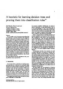
Figure 2. A Decision Tree Representation and Solution of the MD Problem Utility
Solving a strategy matrix representation is straightforward. For each strategy, we compute its expected utility. Next, we identify an optimal strategy by identifying the maximum expected utility. In the MD problem, the expected utility of each strategy is shown in the last column in Table II. The maximum expected utility is 7.998. Thus the optimal strategy is (t, ~t), i.e., treat if S = s, and not treat if S = ~s.
7.4884
p 5.7593
4.1019
In this section, we describe a decision tree representation and solution of the MD problem. See Raiffa [1968] for a primer on the decision tree representation and solution method.
~t
Decision Tree Representation. Figure 1 shows the preprocessing of probabilities that has to be done before we can complete a decision tree representation of the MD problem. In the probability tree on the left, we compute the joint probability distribution by multiplying the conditionals. For example, Pr(d, p, s) = Pr(d) Pr(p | d) Pr(s | p) = (.10)(.80)(.70) = .0560. In the probability tree on the right, we compute the desired conditionals by additions and divisions.
.80 d .10
S .30 ~s s
P .20 ~p
.20
.90 ~d
.80 ~s s .70
~p
s
.30 ~s s .20
~d d
.3075
.0040
.5106
~p
.0255 .9745
~d d
S .0945
p .0931 .0405 .1530
.6925
~s
.6279
~d d
~p
4.4173
.0560
.0945 .0040
.1530 .0240
.0405 .0160
.0255
D .9745
~d
.9745
d
.3721
~d
.6279
d
.0255
~d
.9745
d
.3721
~d
.6279
d
.0255
~d
.9745
d
.3721
~d
.6279
d
.0255
~d
.9745
.5106
.6120
~s
0
2 1
10 10
D
.9069
6 8
D
t
8.9776
4
D
P ~p
.6925
.0931
8
D
5.6033
p
D
P .9069
.6120
.3721
~d
6
D
P
.3075
7.4884
D
.0160
S .80 ~s
.6279
.0255
S
D
P
S
P .85
.4894 .0240
S
D p .15
d .3721
d
7.9880
Figure 1. The Preprocessing of Probabilities in the MD Problem p
.4894
9.7707
Rollback Method. Starting from the leaves, we recursively delete all random and decision variable nodes in the tree. We delete each random variable node by averaging the utilities at the end of its edges with the probability distribution at that node (“averaging out”). We delete each
.0560
p
~p
Figure 2 shows a complete decision tree representation of the Medical Diagnosis problem. (In Figure 2, the utility values shown in bold are computed during the solution phase and are not part of the representation.) Each path from the root node to a leaf node represents a scenario. This tree has 16 scenarios. The tree is symmetric, i.e., each scenario includes the same four variables S, T, P, and D, in the same sequence STPD.
s .70
.6279
T 1.2558
s
~d
10
D
.5106
t
5.7593
.3721
P ~p
4 DECISION TREES
p
.4894
d
4.1019
T 1.2558
~t
p
.0931
~p
0
D
P 8.9776
4
.9069
2 1
D 9.7707
10
decision variable node by maximizing the utilities at the end of its edges (“folding back”). This method is called rollback. The results of the rollback method for the MD problem are shown in Figure 2.
5 SCENARIO TREES In this section, we describe the scenario tree representation and solution technique. A scenario tree representation of the MD problem is shown in Figure 3. (In Figure 3, the utility values shown in bold are computed during the solution phase and are not part of the representation.) A scenario tree is slightly different from a decision tree. In a scenario tree, we do not have to specify probabilities for each edge emanating from a chance node. Instead we have to specify probabilities for each scenario, i.e., for each
Figure 3. A Scenario Tree Representation and Solution of the MD Problem Path Weighted Utility Probability Utility 1.127
10
.0560
0.560
~d
6
.0945
0.567
d
8
.0040
0.032
~d
4
.1530
0.612
d
0
.0560
0
~d
2
.0945
0.189
d
1
.0040
0.004
~d
10
.1530
1.530
d
10
.0240
0.240
d D
p 1.771
P t
~p
D 0.644
1.771
T 0.189
D
p
~t s
P 1.723
~p
D 1.534
7.988
S 0.483
D
p 3.059
~d
6
.0405
0.243
d
8
.0160
0.128
~d
4
.6120
2.448
d
0
.0240
0
~d
2
.0405
.081
d
1
.0160
.016
10
.6120
P ~s t
~p
D 2.576
T 6.217
0.081
D
p
~t
P 6.217
~p
D 6.136
~d
path from the root node to a leaf node. We call these probabilities path probabilities. For a leaf node, the path probability represents the conditional probability of reaching the leaf node conditional on a DM’s strategy that makes the leaf node reachable. This probability is simply the conditional probability of all events on the path conditional on all acts on the path. For example, the probability of the top-most path in the scenario tree of Figure 3 is Pr(S = s, P = p, D = d | T = t). Let 6 denote the set of all scenarios. Consider the probability function p: 6 ® [0, 1] that assigns the path probability p(x) to each scenario x Î 6. We call the function p the path probability function. Consider a strategy y available to the DM. We can encode y as a function xy: 6 ® {0, 1}such that xy(x) = 0 if scenario x has a zero probability of occurring, and xy(x) = 1 otherwise. We call xy a strategy function corresponding to strategy y. Given a strategy function xy, we can define
the product pÄxy as the function pÄxy: 6 ® [0, 1] such that (pÄxy)(x) = p(x) xy(x) for each x Î 6. A path probability function p has the following property. If y is a strategy, then pÄxy is a probability distribution function, i.e., S {(pÄxy)(x) | x Î 6} = 1. Let u: 6 ® R denote the utility function, i.e., u(x) is the DM’s utility under scenario x. Consider the product pÄu: 6 ® R defined as follows: (pÄu)(x) = p(x) u(x) for all x Î 6. We call pÄu the weighted utility function. If the DM chooses strategy y, then the DM’s expected utility is S{((pÄxy)Äu)(x) | x Î 6}. Notice that (pÄxy)Äu = (pÄu)Äx y. Thus the problem can be stated as follows: Find strategy y so as to maximize S{((pÄu)Äxy)(x) | x Î 6}. The pruning method that we will now describe solves precisely this problem using deterministic dynamic programming. The Pruning Method. First, for each leaf node, we compute the weighted utility by multiplying the utility and the path probability. Hence forth, we use the weighted utilities for pruning chance and decision nodes. Pruning Chance Nodes. If we have a chance node all of whose edges end in leaf nodes, first we compute the sum of the weighted utilities at the end of its edges, and next we replace the subtree associated with the chance node by a payoff node whose value is set equal to the computed sum of weighted utilities.
Pruning Decision Nodes. If we have a decision node all of whose edges end in payoff nodes, first we compute the maximum of the weighted utilities, and next we replace the subtree associated with the decision node by a payoff node whose value is set at the computed maximum value of weighted utilities. Each time we prune a decision node, we keep track of a value of the decision node where the maximum is achieved. 6.12
When we have pruned all decision nodes, we have an optimal strategy. When we have pruned all decision and chance nodes, we end with one payoff node whose utility value is the expected utility of an optimal strategy. This pruning method is illustrated in Figure 3.
6 GAME TREES The game tree representation technique for decision problems is described in [Shenoy 1993b]. It is based on von Neumann and Morgenstern’s [1944] extensive form representation of n-person games. Figure 4 shows a game
of node T. In information set I1, the physician knows that S = s, but not the values of D and P. In information set I2, the physician knows that S = ~s, but not the values of D and P. In game trees, the sequence of variables on a Game trees are similar in many ways to decision trees. path from the root node to a leaf node need not represent The main difference between the two representation information constraints. Instead, the sequence may techniques is the encoding of information constraints. In represent time, causation, etc. If we have a causal decision tree, information constraints are encoded in the probability model (as we do in the MD problem), and we sequencing of chance and decision nodes in each scenario. use the sequence to represent causation, then no Thus if the value of a chance variable R is known to the preprocessing is required to represent a decision problem decision maker when she chooses a value of a decision as a game tree. In Figure 4, for example, all the variable N, then R must precede N on the paths from the probabilities on edges are specified in the statement of the root node to leaf nodes. In game trees, information MD problem. constraints are encoded by information sets. Information The Rollback Method for Game Trees. The sets are a partition of the set of decision nodes in a game decision tree rollback method generalizes to game trees tree. When faced with a decision, a decision maker knows [Shenoy 1993b]. We start from the neighbors of payoff which information set she is in, but does not know which nodes and go toward the root until the entire tree has been node in an information set she is at. In Figure 4, there are pruned. The rule for pruning chance nodes is exactly the two information sets I1 and I2 each containing 4 instances same as in the rollback procedure of decision trees. The rule for pruning decision nodes is slightly Figure 4. A Game Tree Representation and Solution of the MD different from the rollback procedure of decision Problem trees. tree representation of the MD problem. (In Figure 4, the utilities shown in bold are computed during the solution phase and are not part of the game tree representation.)
I1
t
Utility 10
10
T s 7
~t S
I2 ~s
p
0.7
0.8 0
6.08
t
0.3
0 10
T ~t t
P
0 8
8
~p
T
0.2 s
d
0.2 ~t
0.1 2.4
1
S t ~s
0.8 1
8
T
7.988
~t t
D
1 6
6
T s 4.8
~d
0.9
0.7 ~t t
~s p 8.2
0.3
0.15
2
~t t 4
0.85 s
2 4
T
0.2 ~t
8.8
6
T
P ~p
2
S
10
S t ~s
0.8 10
4
T ~t
10
Suppose we have an information set such that the edges leading out of the decision nodes end at payoff nodes. First, we compute the conditional probability distribution on the decision nodes of the information set conditioned on the event that we have reached the information set (the details of this step are explained in the following paragraph). Second, for each value of the decision variable associated with the information set, we compute the expected payoff using the payoffs at the end of corresponding edges and using the conditional distribution computed in the first step. Third, we identify a value of the decision variable (and the corresponding edges of each decision node) associated with the maximum expected payoff. Fourth, we prune each decision node by replacing the corresponding subtree by a payoff node whose payoff is equal to the payoff at the end of its edge identified in step 3. We call this technique (for pruning decision nodes in an information set) pruning by maximization of conditional expectation. Pruning by maximization of conditional expectation generalizes the method of pruning a singleton information set by maximization. Computing the conditional distribution for an information set is easy. For each decision node in the information set, we simply multiply all probabilities on the chance edges in the path from the root to the decision node. This gives an unconditional distribution on the nodes in the information set. The sum of these probabilities gives us the probability of reaching the information set assuming prior decisions that allow us to get there. To compute the conditional distribution, we normalize this unconditional distribution by dividing by the sum of the probabilities. From a
the weighted utilities is 0 + .004 + 0.189 + 1.530 = 1.723. Since 1.771 > 1.723, we identify edge T = t with each node in I1. The results of executing the pruning method for the MD game tree are shown in Figure 5.
computational perspective, the normalization step is unnecessary and can be dispensed with. We will illustrate pruning decision nodes by conditional expectation for the game tree representation of the MD problem. Consider information set I1 in Figure 4. Notice that all four decision nodes in I1 have edges leading to payoff nodes. The unnormalized distribution for the three nodes in I1 (from top to bottom) is given by the probability vector (0.1*0.8*0.7, 0.1*0.2*0.2, 0.9*0.15*0.7, 0.9*0.85*0.2) = (0.0560, 0.0040, 0.0945, 0.1530). Thus for T = t, the (unnormalized) expected payoff is (0.0560 *10) + (0.0040*8) + (0.0945*6) + (0.1530*4) = 1.771, and for T = ~t, the expected payoff is (0.0560*0) + (0.0040*1) + (0.0945*2) + (0.1530*10) = 1.723. Since 1.771 > 1.723, we identify edge T = t with each node in I1. The rollback method is illustrated in Figure 4. The Pruning Method for Game Trees. Next, we describe a generalization of the pruning method described in the previous section so that it applies to game trees. First, we compute path probabilities and weighted utilities for all payoff nodes. The rule for pruning chance nodes is exactly the same as in decision trees. The rule for pruning decision nodes is as follows. Pruning Decision Nodes. Suppose we have an information set such that the edges leading out of the decision nodes end at payoff nodes. First, for each value of the decision variable, we compute the sum of the weighted utilities at the end of the respective edges of the decision nodes in the information set. Second, we identify a value of the decision variable that has the maximum sum of weighted utilities computed in the first step. Third, we prune each decision node by replacing the corresponding subtree by a payoff node whose value is equal to the weighted utility at the end of its edge corresponding to the value of the decision variable identified in the second step. We will illustrate the method for pruning decision nodes in game trees using the MD problem. Consider decision nodes in information set I1. For T = t, the sum of the weighted utilities is 0.560 + 0.032 + 0.567 + 0.612 = 1.771, and for T = ~t, the sum of
The correctness of this method follows from exactly the same arguments as in the case of scenario trees. The computational efficiencies of the rollback method and the pruning method are compared in the next section.
7 COMPARISON In this section, we compare scenario trees and game trees to strategy matrices and decision trees. Also we compare the pruning method of scenario trees and game trees to the rollback method of decision trees and game trees. Strategy Matrices. The strategy matrix representation involves considerable preprocessing. Not only do we have to compute the joint probability distribution of all chance
Figure 5. The MD Game Tree Solved Using the Pruning Method I1
t
Path Weighted Utility Probability Utility 0.0560 0.560 10
0.560
T s 0.560
0.0560
0
I2
t
10
0.0240
0.240
~t t
0
0.0240
0
8
0.0040
0.032
~t
1
0.0040
0.004
t
8
0.0160
0.128
~t t
1
0.0160
0.016
6
0.0945
0.567
~t
2
0.0945
0.189
t
6
0.0405
0.243
2
0.0405
0.081
4
0.1530
0.612
10
0.1530
1.530
4
0.6120
2.448
10
0.6120
6.120
0.3
0.8 0
0.608
0
~t S ~s
p
0.7
T
P 0.032
~p
T
0.2 s
d
0.1 0.048
0.2
S ~s
0.8 0.016
T
7.988
D 0.567
T s 0.648
~d
0.9
S ~s
p 7.380
0.7
0.3
0.15
0.081
T ~t t
P ~p
0.612
0.85 s
T
0.2 ~t
6.732
S t ~s
0.8 6.120
T ~t
variables, we also have to identify all possible strategies. The number of configurations in the frame of all chance variables is an exponential function of the number of chance variables, and the number of strategies is an exponential function of the number of decision nodes in a decision tree. Thus, representation and solution of strategy matrices involve global computation (on the space of configurations of all chance variables) to compute the joint probability distribution, and global computation (on the space of all strategies) to compute an optimal strategy. Strategy matrices have some advantages. They can be used to define optimal strategies. Also, the solution method of strategy matrices yields not only the utility of an optimal strategy but also the utilities of all strategies. For example, in the MD problem, the strategy (~t, ~t) has a utility of 7.940 that is only marginally lower than the utility of the optimal strategy.
Figure 6. Computing the Conditional Probability Distributions Using the Arc Reversal Method Initial influence diagram: D
P
S
Numerical details of arc reversal
After reversing arc D ®P: D
P
S
.10
P
In the MD problem, representation and solution of the strategy matrix (shown in Table II) involves a total of 75 operations (where we count each addition, multiplication, division, and comparison as an operation). A breakdown is as follows. Computing the joint probability distribution involves 12 operations, and computing the maximum expected utility involves 63 operations (15 operations to compute the expected utility of each strategy and 3 operations to identify the maximum). In general, suppose we have a symmetric decision problem with m chance variables each of which has 2 values, with n decision variables each of which has 2 values, and with 2k distinct strategies1. Then representing and solving the problem using the strategy matrix method requires a total of approximately 2m+k+1 + 2m+1 operations (approximately 2m+1 to compute the joint probability distribution, 2m+1 – 1 to compute the expected utility of each strategy, and approximately 2k to identify an optimal strategy). Decision Trees. The decision tree representation requires conditional probability distributions for each chance node in a decision tree. If we compute the conditional probability distributions from the joint probability distribution (as described in Figure 1), then this involves global computation on the space of all
1 k denotes, for example, the number of decision nodes in a decision tree representation, or the number of information sets in a game tree representation. The value of k depends on the information constraints. It can be easily shown that 2n – 1 £ k £ 2m+n – 2m.
S
.3721
p
.20 . 020 ~p
.2150
D
.6279
~d
.080 .135
P .90 ~d
D
P
D
d
p . 135 .15 P
p S .2150
After reversing arc P®S:
d
p . 080 .80
d
.7850
.85 . 765 ~p
~p
D
.9745
~d
s . 1505 .70
p s .3075
.30 . 0645 ~s
P
.0255
.4894
P
.5106
~p
.020 .765 .1505 .1570
S .7850 S ~p
s . 1570 .20 .80 . 6280 ~s
p .6925
~s
.0931
P
.9069
~p
.0645 .6280
configurations. The rollback method however computes an optimal strategy using local computation. In the MD problem, representation and solution of the decision tree (shown in Figure 2) involve a total of 71 operations. A breakdown of the total is as follows. Computing the conditional probability distributions as shown in Figure 1 involves 30 operations, and executing the rollback method as shown in Figure 2 involves 41 operations (3 operations for each of the chance nodes and 1 operation for each of the decision nodes). The decision tree representation and solution technique can be made more efficient as follows. First, we can use the arc-reversal method [Olmsted 1983, Shachter 1986] to compute the conditional probability distributions. The arcreversal method uses local computation. This is illustrated in Figure 6. Only 20 operations are needed to compute the requisite conditionals using the arc-reversal method. Second, the decision tree solution can be made more efficient by identifying coalescence [Olmsted 1983]. In the MD problem, by using coalescence, we can simplify the decision tree as shown in Figure 7. The rollback method can be executed for the coalesced decision tree using only 23 operations (3 operation for each chance node and 1 operation for each decision node). Thus by using the arcreversal method and coalescence, we can represent and solve the MD problem using only 43 operations. We are assuming here that identifying coalescence is done during the representation phase by the modeler. In general, automating coalescence in decision trees is not easy. However, coalescence is automatically achieved in influence diagrams and valuation networks [Shenoy 1994]. In influence diagrams and valuation networks, coalescence is achieved by local computation. The arc-reversal method
Figure 7. A Decision Tree Representation and Solution of the MD Problem Using Coalescence p
.4894
5.7593
P ~p
t
.5106
5.7593
.3075
Utilities
T
p
~t
.4894
7.4884
d .3721
10
~d .6279
6
D
P
s 5.6033
~p
d
.5106
.0255
8
4.1019 D
~d .9745
7.988
4
S d p
.0931
1.2558
.3721
0
D ~d .6279
4.4173
2
P d
~s
~p
.9069
t
.0255 9.7707
1
D ~d .9745
.6925
10
T
8.9776
p
~t
.0931
P 8.9776
~p
chance nodes, and 2m+n leaf nodes. Suppose that the decision tree representation has approximately the same number of decision and chance nodes, say 2m+n–1 chance nodes and 2m+n–1 decision nodes. Then the rollback method would require a total of approximately 2m+n+1 operations (3 operations to prune each chance node and 1 operation to prune each decision node), and the pruning method would require a total of approximately 2m+n+1 + 2m+1 operations (2m+1 to compute the joint probability distribution, 2m+n to compute the weighted utilities, 1 operation to prune each chance node and 1 operation to prune each decision node). In this case, the rollback method is more efficient than the pruning method.
.9069
of influence diagrams solves the MD problem using 43 operations, and the fusion algorithm of valuation networks [Shenoy 1992, 1993a] solves the MD problem using 31 operations [Shenoy 1994]. Scenario Trees. Scenario trees do not require conditional probability distributions. However, we do require path probabilities. In the MD problem, computation of the path probabilities is achieved by computing the joint distribution of all chance variables. This involves 12 operations. Executing the pruning method for the scenario tree representation shown in Figure 3 involves a total of 31 operations (16 operations to compute the weighted utilities, and 1 operation per decision and chance node). Thus a total of 43 operations are required to represent and solve the MD problem using the scenario tree method. In general, the scenario tree method involves working on the global space of all configurations. Unlike decision trees, we cannot use either arc-reversal or coalescence to make the representation and solution more efficient. The pruning method of scenario trees does use local computation to identify an optimal strategy and compute its utility. Suppose that we have a symmetric decision problem with m chance variables and n decision variables, suppose that each variable has two values, and suppose that all conditional probabilities required in the decision tree representation are specified in the problem. A decision tree representation would have a total of 2m+n – 1 decision and
Now suppose that we have the same decision problem as above except that Bayesian revision of probabilities is required before the problem can be represented as a decision tree. In this case, if we compute the required conditionals by computing the joint, this would require a total of approximately 2m+n+1 + 2m+2 + 2m operations (2m+1 operations to compute the joint, 2m+1 + 2m operations to compute the required conditionals, and 2m+n+1 operations for rollback). If we use a scenario tree representation with the pruning method, then we would need a total of approximately 2m+n+1 + 2m+1 operations (2m+1 to compute the joint probability distribution, 2m+n to compute the weighted utilities, and 2m+n operations to prune the nodes). In this case, the scenario tree representation with the pruning method is more efficient than the decision tree with the rollback method. Game Trees. If we assume that we have a causal probability model for all chance variables, then unlike strategy matrices, decision trees, and scenario trees, game trees do not require any preprocessing. Executing the rollback method for the MD game tree (see Figure 4) requires 63 operations (12 to compute conditional probabilities of reaching decision nodes in information sets, 15 operation to prune each information set, and 3 operations to prune each chance node). In comparison, executing the pruning method for the MD game tree (see Figure 5) requires only 49 operations (12 operations to compute the path probabilities, 16 operations to compute the weighted utilities, 7 operations to prune the decision nodes in each of 2 information sets, and 1 operation to prune each of 7 chance nodes). In general, suppose we have a game tree with m chance variables each of which has 2 values, with n decision variables each of which has 2 values, with 2m+n–1 chance nodes, and with 2m+n–1 decision nodes in k information sets. If we use the rollback method to solve the game tree, we would need a total of approximately 2m+n+1 + 2m+n + 2m+n–1 + 2m+1 operations (2m+1 operations to compute the unnormalized conditional probability distributions at each information set, 2m+n+1 to prune the k information sets, and 3(2m+n–1) operations to prune the 2m+n–1 chance nodes). If we use the pruning method described in this paper, then we need a total of approximately 2m+n+1 + 2m+n–1 + 2m+1 operations (2m+1 operations to compute the path probabilities, 2m+n operations to compute the weighted utilities, 2m+n to prune the k
Table III. A Comparison of Computational Efficiency of Different Techniques for the MD Problem # Operations (+, ´, ¸, ³) Representation in MD Problem (Preprocessing) Strategy Matrix with Expected Values Decision Tree with Rollback Scenario Tree with Pruning Game Tree with Rollback Game Tree with Pruning Influence Diagram with Arc Reversal
generalizes to game trees and it is more efficient than the rollback method for game trees.
Solution
TOTAL
12
63
75
I am grateful to Rui Guo for comments and discussions.
30
41
71
References
12
31
43
0
63
63
Acknowledgments
Luce, R. D. and H. Raiffa (1957), Games and Decisions: Introduction and Critical Survey, John Wiley & Sons, New York, NY.
Olmsted, S. M. (1983), “On representing and solving decision problems,” Ph.D. thesis, Department of EngineeringEconomic Systems, Stanford University, 0 49 49 Stanford, CA. Table IV. A Comparison of Computational Efficiencies of Different Techniques Pearl, J. (1988), Probabilistic Reasoning in Intelligent Problem Representation and Approximate Total # Operations Systems: Networks of Plausible Characteristics Solution Technique (+, ´, ¸, ³) Inference, Morgan Kaufmann, San Mateo, CA. Strategy Matrix m+k+1 m+1 General with Expected Values 2 +2 Raiffa, H. (1968), Decision Analysis, Addison-Wesley, Decision Tree Reading, MA. No Bayesian Revision with Rollback 2m+n+1 Scenario Tree Raiffa, H. and R. Schlaifer No Bayesian Revision with Pruning 2m+n+1 + 2m+1 (1961), Applied Statistical Decision Theory, MIT Press, Decision Tree Cambridge, MA. Bayesian Revision with Rollback 2m+n+1 + 2m+2 + 2m Scenario Tree Shachter, R. D. (1986), Bayesian Revision with Pruning 2m+n+1 + 2m+1 “Evaluating influence diagrams,” Operations Game Tree 2m+n+1 + 2m+n + 2m+n–1 + 2m+1 Research, 34(6), 871-882. General with Rollback Game Tree Shenoy, P. P. (1992), General with Pruning 2m+n+1 + 2m+n–1 + 2m+1 “Valuation-based systems for Bayesian decision analysis,” information sets, and 2m+n–1 operations to prune the Operations Research, 40(3), 463–484. 2m+n–1 chance nodes). Thus the pruning method is more Shenoy, P. P. (1993a), “A new method for representing efficient than the rollback method for game trees. and solving Bayesian decision problems,” in D. J. Hand Table III summarizes the computational efficiencies of the (ed.), Artificial Intelligence Frontiers in Statistics: AI different techniques for the MD problem, and Table IV and Statistics III, 119–138, Chapman & Hall, London. summarizes the computational efficiencies of the different Shenoy, P. P. (1993b), “Game trees for decision techniques in general analysis,” Working Paper No. 239, School of Business, University of Kansas, Lawrence, KS. An 8-page summary 8 CONCLUSION of this paper appeared as “Information sets in decision The main objective of this paper was to introduce a new theory,” in M. Clarke, R. Kruse and S. Moral (eds.), pruning method to solve decision trees and game trees. In Symbolic and Quantitative Approaches to Reasoning and decision problems requiring Bayesian revision of Uncertainty, Lecture Notes in Computer Science No. probabilities for a decision tree representation, the new 747, 1993, 318–325, Springer-Verlag, Berlin. pruning method suggests a slight variant of decision trees Shenoy, P. P. (1994), “A comparison of graphical that we call scenario trees. For such problems, the techniques for decision analysis,” European Journal of scenario tree representation with the pruning method is Operational Research, 78(1), 1–21. more efficient than the decision tree representation with the rollback method (assuming we compute the conditionals from the joint). The pruning method 0
49
49
von Neumann, J. and O. Morgenstern (1944), Theory of Games and Economic Behavior, 1st edition, Princeton University Press, Princeton, NJ.