Journal of Mathematical Finance, 2014, 4, 207-219 Published Online May 2014 in SciRes. http://www.scirp.org/journal/jmf http://dx.doi.org/10.4236/jmf.2014.43018
A New Range-Based Regime-Switching Dynamic Conditional Correlation Model for Minimum-Variance Hedging Yi-Kai Su1*, Chun-Chou Wu2 1
Graduate Institute of Finance, National Taiwan University of Science and Technology, Taiwan Department of Finance, National Kaohsiung First University of Science and Technology, Taiwan * Email:
[email protected],
[email protected]
2
Received 5 March 2014; revised 7 April 2014; accepted 7 May 2014 Copyright © 2014 by authors and Scientific Research Publishing Inc. This work is licensed under the Creative Commons Attribution International License (CC BY). http://creativecommons.org/licenses/by/4.0/
Abstract This study proposes a new range-based Markov-switching dynamic conditional correlation (MSDCC) model for estimating the minimum-variance hedging ratio and comparing its hedging performance with that of alternative conventional hedging models, including the naïve, OLS regression, return-based DCC, range-based DCC and return-based MS-DCC models. The empirical results show that the embedded Markov-switching adjustment in the range-based DCC model can clearly delineate uncertain exogenous shocks and make the estimated correlation process more in line with reality. Overall, in-sample and out-of sample tests indicate that the range-based MS-DCC model outperforms other static and dynamic hedging models.
Keywords Minimum-Variance Hedge Ratio, Markov-Switching, Correlation, Range-Based DCC Model, Regime Shift
1. Introduction The dynamic conditional correlation (DCC) model, the celebrated multivariate correlation estimation model proposed by Engle [1], solves the requirement of a positive definite constraint in parameter estimation, the ability to estimate many parameters and time-varying correlation1. The DCC model also provides some advantages *
Corresponding author. The generalization of the univariate volatility models to the multivariate case is the VECH model, introduced by Bollerslev et al. [2]. However, the VECH model has some disadvantages, including problems determining a positive definite and the possibility of including too many parameters. In response, Engle and Kroner [3] propose the BEKK model to guarantee a positive definite constraint. However, the BEKK model still has the problem of facing too many parameter estimations for higher dimensional systems. Although the VECH and BEKK model have some drawbacks, they are more flexible than the constant correlation model in allowing time-varying covariance (Bollerslev, [4]). 1
How to cite this paper: Su, Y.-K. and Wu, C.-C. (2014) A New Range-Based Regime-Switching Dynamic Conditional Correlation Model for Minimum-Variance Hedging. Journal of Mathematical Finance, 4, 207-219. http://dx.doi.org/10.4236/jmf.2014.43018
Y.-K. Su, C.-C. Wu
through its operating procedure, which enables more parsimonious parameter estimation and easy estimation. Drawing on related literatures, the current models of correlation estimation were developed to extract return data to estimate covariance processes. A few recent studies have attempted to introduce a range variable to replace the return variable for more information content and to account for efficient market theory. More information can be gathered with a range structure than with a return variable when estimating a volatility model for many separate empirical results2. For example, Chou et al. [12] construct a range-based DCC model and propose that their model setting outperforms the original return-based DCC model in estimating and forecasting covariance matrices. Although the return- and range-based DCC models feature many advantages in correlation process fitting, they still place several constraints on linear parameters for covariance and correlation equations3. It is natural to introduce a nonlinear mechanism into the return- and range-based DCC models to enhance feasibility. In this study, we propose a new range-based regime-switching DCC model that is able to enhance the hedge effect in futures markets. Conventional approaches to nonlinear adjustment among financial time-series models include threshold autoregressive techniques, smooth transition and Markov-switching. We introduce the Markov-switching method proposed by Hamilton [15] [16] to extend the original DCC structure. One advantage of the Markov-switching method is that it treats the regime shift as an exogenous variable. Simplifying the formidable task of statistical estimation, the Markov-switching structure can be applied from the mean to variance and covariance equations. The combination Markov-switching and volatility model is able to address volatility processes with greater flexibility through regime-switching. Meanwhile, such a volatility model with Markov-switching can enable the estimated coefficients to change in different states. Drawing on the DCC model of Engle [1], the extension of a return-based DCC model with regime-switching has been introduced in some studies. For instance, Pelletier [17] and Billio and Caporin [18] propose a variant multivariate GARCH model composed of a Markov chain and the DCC model. These studies consider a solution that a discrete level shift may exist in the dynamic conditional correlation process. Moreover, they verify that the return-based Markov-switching DCC model outperforms Engle’s [1] single-regime DCC model structure. Because the range-based DCC model is superior to the conventional return-based method in depicting the pattern of correlation shown by Chou et al. [12], it is necessary to explore whether the range correlation model with data structure change remains useful for futures hedging. Accordingly, we construct a Markov chain structure into the range-based DCC model, and compute the minimum-variance hedge ratio for comparison with other hedging approaches. The literature has historically used the utility function and ordinary least squares model to discuss minimum-variance hedging. According to Chen et al. [19] and Lien and Tse’s [20] research, advanced econometric models have recently been used to measure the minimum-variance hedge ratio. In other words, the manner of hedging is shifting from static hedging to time-varying hedging. There is a large body of evidence showing that time-varying hedging approaches perform better than the static case4. In contrast, some empirical studies argue that there are no significant improvements from employing advanced econometric techniques5. According to Lien [29]-[31], the inconsistent performance of such hedging is caused by the abuse of hedging effectiveness measures. This proposal is supported by Ederington [32]. From previous discussions, there remains a difficulty in using advanced econometric tools to measure the hedge ratio. Therefore, this study employs a range-based Markov-switching dynamic conditional correlation (MS-DCC) model to estimate the dynamic hedge ratio and discusses the hedging effectiveness of other approaches. The rest of this article is organized as follows. In the next section, the range-based regime-switching DCC model is introduced, and minimum-variance hedging is described in the following section. In the fourth section, this study presents a hedging effectiveness measurement. The empirical results and the economic intuition of these results are reported in the fifth section. The final section provides the conclusion.
2. Range-Based Regime-Switching Dynamic Conditional Correlation Model To introduce the regime-switching structure to the range-based dynamic conditional correlation process, the range-based MS-DCC model with a general S-regime can be expressed as: 2
Also see Parkinson [5], Rogers and Satchell [6], Yang and Zhang [7], Alizadeh, et al. [8], Brandt and Jones [9], Chou [10] [11], Chou, et al. [12] and Cai, et al. [13]. 3 Also see Danielsson [14]. 4 See also Baillie and Myers [21], Kroner and Sultan [22], Tong [23], Choudhry [24] and Alizadeh and Nomikos [25]. 5 See also Lien, et al. [26], Copeland and Zhu [27] and Alexander and Barbosa [28].
208
Y.-K. Su, C.-C. Wu
t −1 ~ exp (1, ⋅) , k 1, 2. u= k ,t | I
Rk ,t λk ,t uk ,t =
(1a)
λk ,t = ωk + α k Rk ,t −1 + β k λk ,t −1 ,
(1b)
adjk × λk ,t , ηk ,t = rk ,t λk*,t , where λk*,t =
adjk = σ k λˆk ,
(1c)
= pij Pr = st −1 i ) , = i, j 1, , S . ( st j=
(1d)
Qtij =(1 − A j − B j ) Q j + A jηt −1ηt′−1 + B j Qti−1 ,
(1e)
{ }
Γ ijt = diag Qtij
−1 2
{ }
Qtij diag Qtij
−1 2
,
(1f)
where Equations (1a)-(1c) represent the range-based volatility specification, Rk ,t denotes the observed high-low range in the logarithm of the kth asset during the time interval t, λk ,t denotes the conditional mean of the range,
uk ,t denotes the disturbance term, which follows the exponential distribution with unit mean, ηk ,t = rk ,t λk*,t is
(λ ) * k ,t
the standardized residual, and the scaled expected range
is substituted for the conditional standard devi-
ation. The unconditional standard deviation of the return series k and the sampling mean of the estimated conditional range of the series k are represented as σ k and λˆk , respectively. The Markov chain transition probaS
bility, which has the constraints
∑ pij = 1 j =1
for i = 1, 2, , S , and 0 ≤ pij ≤ 1 for i, j = 1, 2, , S , is shown in
Equation (1d). It is intuitive to define the stationary distribution of the Markov chain as π ∞st by the time-varying transition probabilities. The dynamic conditional covariance and correlation process with the Markovswitching property are reported in Equations (1e) and (1f). The unconditional correlations can be 1 T represented as Q j = ∑ηtηt′ , a time-varying correlation matrix is denoted by Γ tij , and Qtij denotes a T i =1 time-varying covariance matrix. In Equations (1e) and (1f), the superscript symbol represents the regime shift from i to j. In short, the range-based MS-DCC model is composed of the conditional autoregressive range (CARR) model for the conditional variance process and the Markov-switching approach for the conditional covariance and correlation case. The log likelihood function of the MS-DCC model is presented in this section. According to Engle [1] and Chou et al. [12], the two-step quasi-maximum likelihood approach is suitable for estimating the models in the DCC family. It is natural to execute the first step quasi-maximum likelihood estimation (QMLE) using Equation (2), as our specification allows only the conditional correlation to change in different regimes. The likelihood function of the volatility component, LV (κ ) , can be shown as: 2 rk2,t 1 LV (κ ) = − ∑∑ log ( 2π ) + log λk*,t + *2 2 t k =1 λk ,t
( )
(2)
By maximizing the QMLE of Equation (2), the parameters κ = {ωk , α k , β k } can be estimated and obtained. Using the above-estimated results to the second step of the estimation, the estimation procedure can be finished as shown below: 1) given the filtered probabilities as inputs, determine the joint probabilities as:
(
)
(
Pr st =j , st −1 =i | I t −1 =Pr ( st =j , st −1 =i ) × Pr st −1 =i | I t −1
2) evaluate the regime-dependent log likelihood as:
(
)
(
( )
)
( )
1 T L Rt | λt , st = j , st −1 = i, I t −1 = − ∑ log Γ tij + ηt′ Γ tij 2 t =1
i, j =1, , S
−1
ηt
)
(3)
(4)
3) evaluate the log likelihood of observation t as:
(
) ∑∑ L ( R | λ , s
L Rt | λt , I t −1 =
S
S
=j 1 =i 1
t
t
t
209
)
(
= j , st −1 = i, I t −1 × Pr st = j , st −1 = i | I t −1
)
(5)
Y.-K. Su, C.-C. Wu
(
= L ( Rt , , R1 ) L ( Rt −1 , , R1 ) + L Rt | λt , I t −1
)
(6)
4) renew the joint probabilities as:
(
t −1
(
)
( )
L Rt | λt , st = j , st −1 = i, I t −1 × Pr st = j , st −1 = i | I t −1
)
I = st j= Pr , st −1 i | =
(
L Rt | λt , I
t −1
)
(7)
5) calculate the filtered probabilities as:
(
) ∑ Pr= (s S
Pr | It st j= =
t
i =1
)
, st −1 i | I t = j= j 1, , S
(8)
6) renew the dynamic conditional correlation matrix through the following approximation:
( st ∑ Pr=
)
S
Qt j =
i =1
, st −1 i | I t × Qtij j=
(
)
Pr st = j | I t
(9)
7) iterate 1 to 6 until the end of the sample. The unknown parameters of MS-DCC model can be obtained with these estimation procedures.
3. Minimum-Variance Hedging Minimum-variance hedging is the determination of the number of futures contracts against one spot asset that will ensure the minimum variance of the hedging portfolio. Furthermore, minimum-variance hedging can be calculated as a ratio of the covariance of spot-futures returns over the variance of futures returns, namely,
δ* =
cov ( ct , ft )
(10)
var ( ft )
where ct and ft are the spot and futures returns at time t. As the covariance and variance estimates are time varying, Equation (10) can be extended to be the time-varying hedge ratio as:
δ t* =
covt ( ct , ft ) vart ( ft )
.
(11)
This study selects six various minimum-variance hedge ratios for the time being: 1) Naïve: A simple hedging strategy assigning the hedge ratio equal to −1 at all times. 2) OLS: A conventional method for analyzing the minimum-variance hedge ratio, used by Ederington [32] through the simple OLS regression, ct =+ γ δ * ft + ε t .
(12)
The estimated slope, δˆ* , is a constant hedging ratio. 3) Return-based DCC: A classical time-varying correlation model proposed by Engle [1], which can be shown as:
= rk ,t
= hk ,t ε k ,t ε k ,t | I t −1 ~ N ( 0, hk ,t ) , k 1, 2
hk ,t = ωk + α k ε k2,t −1 + β k hk ,t −1 ,
ηk ,t = rk ,t
hk ,t ,
Qt = (1 − A − B ) Q + Aηt −1ηt′−1 + BQt −1 , Γ t = diag {Qt }
−1 2
Qt diag {Qt }
−1 2
(13)
,
4) Range-based DCC: A range-based dynamic conditional correlation model developed by Chou et al. [12], which can be expressed as:
210
Y.-K. Su, C.-C. Wu
uk , t = | I t −1 ~ exp (1, ⋅) , k 1, 2
= Rk ,t λk ,t uk ,t
λk ,t = ωk + α k Rk ,t −1 + β k λk ,t −1 , η k ,t = rk ,t λk*,t , where λk*,t =× adjk λk ,t , adjk = σ k λˆk , Qt = (1 − A − B ) Q + Aηt −1ηt′−1 + BQt −1 , Γ t = diag {Qt }
−1 2
Qt diag {Qt }
−1 2
(14)
,
5) Return-based MS-DCC: A more flexible return-based dynamic conditional correlation model proposed by Pelletier [17] and Billio and Caporin [18], which can be expressed as: = rk ,t
= ε k ,t | I t −1 ~ N ( 0, hk ,t ) , k 1, 2 hk ,t ε k ,t
ωk + α k ε k2,t −1 + β k hk ,t −1 , hk ,t = ηk ,t = rk ,t
hk ,t ,
= pij Pr = st i ) , ( st j=
= i, j 1, , S .
(15)
Qtij =(1 − Aj − B j ) Q j + Ajηt −1ηt′−1 + B j Qti−1 ,
{ }
Γ ijt = diag Qtij
−1 2
{ }
Qtij diag Qtij
−1 2
,
6) Range-based MS-DCC: A range-based dynamic conditional correlation model with a regime-switching structure, which can be expressed as Equations (1a)-(1f).
4. Hedging Effectiveness Measure With regard to the hedging effectiveness measure, this study employs the variance reduction and further calculates the percentage variance reduction. In addition, this study calculates the economic benefits including the expected daily utility and the value-at-risk (VaR) estimate. The investor faces the mean-variance expected daily utility function proposed by Kroner and Sultan [22], which can be represented as: ct +1 − δ t*+1 ft +1 . EtU= ( xt +1 ) Et ( xt +1 ) − kVart ( xt +1 ) , where x= t +1
(16)
Et ( xt +1 ) and Vart ( xt +1 ) represent the expected returns and variance, respectively, from the hedged portfolio. The degree of risk aversion is k. The higher expected daily utility shows that the corresponding hedge portfolio provides more economic benefit. With regard to the VaR estimate, it can be computed as:
= VaR w0 E ( xt +1 ) + zα Var ( xt +1 ) ,
(17)
where w0 denotes the initial value of the hedged portfolio, and zα is the α quantile of normal distribution. A higher VaR indicates that the corresponding hedge portfolio leads to a greater reduction in VaR exposure and to more economic benefit. So far, the reference to variance, Vart ( xt +1 ) , is calculated by equal weight to positive and negative returns. Usually, the investor is more concerned about negative losses than about positive gains. It is logical to discuss the hedging effectiveness of downside risk. This study chooses the semi-variance as the measurement of downside risk because it is a measure of the dispersion of the realized portfolio returns that fall below the target return. The semi-variance can be defined as:
{
Semi-variance = E ( min [τ − xt +1 , 0])
2
},
(18)
where τ is the target return, and xt +1 is the realized portfolio return.
5. Empirical Analysis This study selects two stock indices with different weighting schemes for model testing at this stage, namely, the value-weighted S&P 500 index, the equal-weighted NIKKEI 225 index, and their corresponding futures contracts. The sample period is from January 3, 2000 to June 29, 2011 for the empirical study. One goal of this
211
Y.-K. Su, C.-C. Wu
study is to detect using these two different weighted indices whether the range-based MS-DCC model outperforms competing models. The daily high, low, and close price for the S&P 500 and NIKKEI 225 are obtained from Datastream. Descriptive statistics for daily returns and ranges data are reported in Table 1. The spot and futures index volatilities (standard deviation) for the NIKKEI 225 are larger than those for the S&P 500. This finding is in line with equal-weighted stock indices’ property of having higher volatility than value-weighted indices, as equalweighted schemes allocate the same weight to each stock, and small-cap stocks are generally more volatile than their large-cap counterparts. Both markets’ return and range data are found to reject the null hypothesis of normal distribution by the Bera-Jarque criterion. Here, the Bera-Jarque statistics are greater than the chi-squared value with a degree of freedom of 2. Furthermore, the kurtosis test for both markets’ returns reveals fat tails. Therefore, the GARCH and CARR model are, at first glance, capable of fitting the S&P 500 and NIKKEI 225 market trading data. Table 2 expresses the parameter estimation results for the DCC-GARCH (1,1) and DCC-CARR (1,1) models with the futures and spot indices, respectively. According to Engle [34], this study uses the quasi-maximum likelihood estimation to reduce the problem faced in volatility estimation of over heteroskedasticity. The characteristic of return-based and range-based volatility is shown in Panel A of Table 2. Here, the range-based volatility model is more sensitivity than return-based case in capturing volatility transitory shocks. In addition, this study uses the standardized residuals generated from different market data to estimate the parameters of the dynamic conditional correlation structure. Panel B of Table 2 presents clearly dissimilar dynamic correlation processes. Billio and Caporin [18] believe that using two regimes to configure the model will limit any problems of convergence. For this reason, this study focuses on the estimation of the range-based MS-DCC model with two different regimes. The estimated results for the two-state range- and return-based MS-DCC model are reported in Table 3. According to the model specification, the larger coefficient of (1 − Aj − B j ) is defined as the high-correlation regime, and the smaller coefficient of (1 − Aj − B j ) is defined as the low-correlation regime.
The estimated transition probability of remaining in the low-correlation state
( pˆ11 )
is 0.999 for both stock in-
dices; however, the estimated transition probability of remaining in the high-correlation state ( pˆ 22 ) is 0.997 for the S&P 500 and 0.860 for the NIKKEI 225. This finding indicates the probability of transitioning from low to high correlation is lower than that of the reverse. The expected transition period calculated by the estimated transition probability may provide insight into frequency of regime-switching. The expected transition period from low to high correlation (1 (1 − pˆ11 ) ) is approximately 3.97 years for both the S&P 500 and the NIKKEI 225, but the expected transition period from high to low correlation (1 (1 − pˆ 22 ) ) is approximately 1.32 years for the S&P 500 and 0.03 years for the NIKKEI 2256. This finding indicates that the expected transition period from high to low correlation is shorter than that of the reverse and that the correlation is relatively stable in the long term, although shocks may cause the correlation to oscillate violently and move from a low to high state. This study also calculates the steady-state probabilities of the Markov process as a benchmark. The estimated result of the range-based MS-DCC model indicates that the steady-state probability that the correlation of the S&P 500 will move to a low (high) state in the next period is 0.810 (0.190) and that the probability that the correlation of the NIKKEI 225 will move to a low (high) state in the next period is 0.998 (0.002). In brief, the probability of the expected correlation for either stock index moving to a low state is over 80%. With regard to the dynamic correlation process, the high-correlation state has a larger value of Aˆ than the low-correlation state. That is, the high-correlation state features a stronger instant influence term of shocks for the dynamic correlation process. Figure 1 further shows the smoothed probability of the low-correlation state estimated by the range-based Markov-switching DCC model for the S&P 500 and NIKKEI 225 indices. The patterns differ substantially between the two stock indices. This difference may be attributed to the corresponding estimated transition probability figures. In addition, this finding is also in line with the inference of the expected transition period, which is shown in Table 3. Figure 1 shows that the estimated time-varying correlation has higher probability of remaining in the low-correlation regime for the NIKKEI 225 spot and futures indices than for the S&P 500. The find6
The calculated transition period is deliberately displayed as an annualized figure for ease of comparison.
212
Y.-K. Su, C.-C. Wu
Table 1. Descriptive statistics for the daily returns and ranges of spot and futures of S&P 500 and of NIKKEI 225 (2000.1.3-2011.6.29). S&P 500
NIKKEI 225
Spot
Futures
Spot
Futures
Return
Range
Return
Range
Return
Range
Return
Mean
−0.004
1.528
−0.004
1.533
−0.023
1.541
−0.023
Range 1.738
Median
0.054
1.235
0.064
1.248
0.004
1.324
0.062
1.432
Maximum
10.957
10.904
13.197
11.639
13.235
13.763
18.812
24.144
Minimum
−9.470
0.239
−10.400
0.000
−12.111
0.236
−14.003
0.256
Std. Dev.
1.361
1.117
1.371
1.124
1.616
0.992
1.677
1.375
Skewness
−0.113
3.049
0.039
3.089
−0.401
3.643
−0.257
5.616
Kurtosis
10.670
18.278
12.837
18.905
9.606
29.130
14.897
58.917
Bera-Jarque
7072.398
32505.10
11624.49
34974.54
5198.131
86370.71
16645.12
381803.60
observation
2882
2883
2882
2883
2816
2817
2816
2817
Notes: The Bera-Jarque is the statistic for normality testing.
Table 2. The estimation of range- and return-based dynamic conditional correlation model of daily spot and futures of S&P 500 and of NIKKEI 225 (2000.1.3-2011.6.29). Univariate:
u k ,t = | I t −1 ~ exp (1, ⋅) , k c, f
= Rk ,t λk ,t uk ,t
range-based
λk ,t = ωk + α k Rk ,t −1 + β k λk ,t −1 , adjk = σ k λˆk ,
* ηk ,t = rk ,t λk*,t , where λ = adjk × λk ,t , k ,t
hk ,t ε k ,t ε k ,t | I t −1 ~ N ( 0, hk ,t ) , k c, f =
rk ,t =
hk ,t =+ ωk α k ε k2,t −1 + β k hk ,t −1
return-based
ηk ,t = rk ,t
Qt = (1 − A − B ) Q + Aηt −1ηt′−1 + BQt −1 ,
DCC:
Γ t = diag {Qt }
S&P 500
Panel A: univariate
ωˆ
αˆ βˆ
hk ,t
Futures GARCH
Qt diag {Qt }
−1 2
NIKKEI 225
Spot CARR
−1 2
CARR
Spot
GARCH
CARR
Futures GARCH
CARR
GARCH
0.022
0.013
0.021
0.016
0.031
0.041
0.038
0.046
(0.006)
(0.006)
(0.005)
(0.007)
(0.008)
(0.011)
(0.009)
(0.012)
0.169
0.079
0.178
0.083
0.168
0.109
0.175
0.105
(0.013)
(0.012)
(0.013)
(0.012)
(0.020)
(0.020)
(0.020)
(0.018)
0.816
0.912
0.808
0.907
0.812
0.877
0.803
0.880
(0.014)
(0.011)
(0.014)
(0.011)
(0.022)
(0.019)
(0.023)
(0.017)
Panel B:
S&P 500
NIKKEI 225
DCC
Range-based
Return-based
Range-based
Return-based
Aˆ Bˆ
0.136 (0.010)
0.015 (0.001)
0.046 (0.002)
0.039 (0.001)
0.229 (0.031)
0.980 (0.002)
0.945 (0.002)
0.955 (0.002)
Notes: The number in parentheses is robust standard error proposed by Bollerslev and Wooldridge [33].
ing that the high-correlation regime follows major financial events, especially in the case of the S&P 500, makes intuitive sense7. 7
These financial events include the 2000 technology bubble, the September 11 terrorist attacks, the 2002 stock market crash, the 2007 subprime housing crisis and the 2009 credit crisis.
213
Y.-K. Su, C.-C. Wu
Table 3. The estimation of range- and return-based markov switching dynamic conditional correlation model for daily spot and futures of S&P 500 and NIKKEI 225 (2000.1.3-2011.6.29). Univariate:
t −1 uk ,t | I= ~ exp (1, ⋅) , k c, f
= Rk ,t λk ,t uk ,t
Range-based
λk ,t = ωk + α k Rk ,t −1 + β k λk ,t −1 , where λk*,t =× adjk λk ,t , adjk = σ k λˆk ,
ηk ,t = rk ,t λk*,t ,
= hk ,t ε k ,t ε k ,t | I t −1 ~ N ( 0, hk ,t ) , k c, f
= rk ,t
hk ,t =+ ωk α k ε k2,t −1 + β k hk ,t −1
Return-based
ηk ,t = rk ,t
hk ,t
= pij Pr = st i ) , ( st j= Qtij =(1 − Aj − B j ) Q j + Ajηt −1ηt′−1 + B j Qti−1 ,
MS-DCC:
= Γ tij diag = {Qtij } Qtij diag {Qtij } , i, j 1, 2. −1 2
S&P 500 Regime
Low Correlation
−1 2
NIKKEI 225 High Correlation
Low Correlation
High Correlation
Panel A: Range-based
Aˆ
0.052 (0.004)
0.075 (0.001)
0.074 (0.002)
0.335 (0.095)
Bˆ
0.931 (0.007)
0.268 (0.006)
0.906 (0.003)
0.377 (0.131)
pˆ ii
0.999 (0.194)
0.997 (0.077)
0.999 (0.424)
0.860 (0.117)
0.810
0.190
0.998
0.002
πˆ
i ∞
Panel B: Return-based
Aˆ
0.030 (0.001)
0.147 (0.042)
0.043 (0.002)
0.158 (0.012)
Bˆ
0.957 (0.003)
−0.023 (0.083)
0.955 (0.002)
0.373 (0.042)
pˆ ii
0.994 (0.160)
0.879 (0.170)
0.999 (0.085)
0.968 (0.105)
πˆ ∞i
0.954
0.046
0.990
0.010
Notes: The number in parentheses is robust standard error proposed by Bollerslev and Wooldridge [33]. The probability of staying in the low correlation state is p11 , and of staying in the high correlation state is p22 . The stationary regime probabilities, π ∞1 and π ∞2 , are computed by the expression: π ∞1 =(1 − p22 ) ( 2 − p11 − p22 ) and π ∞2 =(1 − p11 ) ( 2 − p11 − p22 ) , respectively.
NIKKEI 225 smoothed probability
S&P 500 smoothed probability 1.00
1.0
0.98 0.8
0.96 0.94
0.6
0.92 0.4
0.90 0.88
0.2 0.86 0.84
0.0 00
01
02
03
04
05
06
07
08
09
10
11
00
01
02
03
04
05
06
07
08
09
10
11
Figure 1. The smoothed probability of low correlation regime for S&P 500 and NIKKEI 225 (2000.1.3 2011.6.29). This figure plots the smoothed probability estimated by range-based Markov-switching dynamic conditional correlation model.
214
Y.-K. Su, C.-C. Wu
Figure 2 displays the estimated time-varying correlations of the return-based MS-DCC, range-based DCC and MS-DCC models for the S&P 500 and NIKKEI 225. For both stock indices, the fluctuating range of time-varying correlation estimated from the range data is wider than that estimated from return data. The largest range of fluctuation is estimated by the range-based DCC model for the S&P 500, but the range-based MS-DCC model estimates the largest range for the NIKKEI 2258. The correlations estimated by the range-based MS-DCC are less volatile than those estimated by the range-based DCC for the S&P 500, but the estimated results are the opposite for the NIKKEI 225. This finding indicates that the use of range data could lead to correlation estimates with a wider range compared to those produced using return data. Furthermore, considering a regime-switching method for the range-based DCC model could make the correlation estimates more flexible, as the regimeswitching method can capture reactions to variation with greater precision. Table 4 reports the in-sample and out-of-sample forecasting performance summary for various measurements of hedging ratios. The degree of risk aversion is assumed to be k = 4 for the expected daily utility function in Equation (18)9. In the case of given parameters for the VaR estimate, the initial value and the quantile of normal distribution are assumed to be w0 = $1m and z0.05 = −1.645 , respectively. The in-sample hedging effectiveness illustrates that the range-based MS-DCC model outperforms competing models for both the S&P 500 and NIKKEI 225 indices in terms of the measure of variance improvement, the daily utility function and VaR estimation. In terms of variance improvement, the percentage of variance reduction from using the range-based MS-DCC model is 95.9588% for the S&P 500 index and 90.4778% for the NIKKEI 225 index. With regard to one of the economic benefits measures, the daily utility of the range-based MS-DCC model is −0.2989 for the S&P 500 and −0.9945 for the NIKKEI 225 index. Furthermore, another measure of economic benefit, VaR, shows that employing a hedging strategy based on the range-based MS-DCC model could reduce losses by approximately 1.789 million dollar for the S&P 500 and by approximately 1.838 million dollar for the NIKKEI 225. Although all of the measurements of in-sample hedging effectiveness demonstrate that the range-based MS-DCC model outperforms the alternative models, it is essential to assess the more realistic performance of out-of-sample hedging effectiveness. A total of 500 observations are used for the out-of-sample forecast. In Panel B of Table 4, all performance criteria indicate that the range-based MS-DCC model tends to outperform competing models for the S&P 500, but that the naïve hedging strategy could show superior hedging effectiveness for the NIKKEI 225. The inconsistent performance between the in-sample and out-of-sample tests is not an anomaly to us, as previous studies have provided explanations for this finding10. However, it is not appropriate to make a conclusion with regard to out-of-sample performance with these empirical results. So far, the use of variance as the proxy for risk has two flaws: trading position and the proxy chosen. It is necessary to discuss the hedging performance of different trading positions to compare hedging methods, as the short and long positions present different hedging performance (see for instance, Cotter and Hanly [38] and Alizadeh, et al. [35])11. Hedgers are concerned with negative losses; therefore, this study uses semi-variance as an alternative risk proxy to replace the variance variable. Figure 3 shows the optimal hedge ratios estimated by the constant OLS, return-based MS-DCC, range-based DCC and MS-DCC models for the S&P 500 and NIKKEI 225. The hedge ratios of the range-based MS-DCC model are more volatile than those of competing models in the case of the NIKKEI 225; however, different outcomes are found in the case of the S&P 500. This finding is consistent with the results shown in Figure 2. Table 5 presents the out-of-sample performance of various hedging ratios in terms of downside risk for the short and long hedgers. In Panel A, all of the effectiveness criteria for the short hedger indicate that the rangebased MS-DCC model is the most effective hedging strategy for the S&P 500. However, the naïve hedging strategy shows the best performance for the NIKKEI 225. This result from Panel A of Table 5 is almost identical to that from Panel B of Table 4, as both of these calculations are based on short hedgers. Comparing Panel A of Table 5 with Panel B of Table 4, the VaR figures calculated from the semi-standard deviation for each hedging strategy are larger than the corresponding half-VaR figures estimated using the standard deviation. 8
The range of fluctuation in the time-varying correlation for S&P 500 is (0.8581, 0.9957) for the range-based DCC, (0.8964, 0.9909) for the return-based MS-DCC, and (0.8947, 0.9932) for the range-based MS-DCC. However, the range of fluctuation in the time-varying correlation for NIKKEI 225 is (0.3597, 0.9915) for the range-based DCC, (0.5083, 0.9910) for the return-based MS-DCC, and (0.2413, 0.9932) for the range-based MS-DCC. 9 This setting of the degree of risk aversion is in line with Alizadeh and Nomikos [25] and Alizadeh et al. [35]. 10 Engel [36] and Marsh [37] clarify that parameter instability may lead to differences between in-sample and out-of-sample performance. 11
The hedge portfolio is calculated as
( +c
t
− δ t* f t ) for short hedger, and as
215
( −c
t
+ δ t* f t ) for long hedger.
Y.-K. Su, C.-C. Wu
S&P 500 time varying correlation
NIKKEI 225 time varying correlation
1.00
1.0
0.98
0.9
0.96
0.8
0.94
0.7
0.92
0.6
0.90
0.5
0.88
0.4
0.86
0.3 0.2
0.84 00
01
02
03
04
05
06
07
08
09
10
00
11
01
02
03
04
05
06
07
08
09
10
11
Corr_MS-DCCC Corr_MS-DCCG Corr_DCCC
Corr_MSDCCC Corr_MSDCCG Corr_DCCC
Figure 2. The estimated time varying correlations for S&P 500 and NIKKEI 225 (2000.1.3-2011.6.29). This figure plots three estimated time varying correlations including range-based DCC (Corr_DCCC), MS-DCC (Corr_MSDCCC) and return-based MS-DCC (Corr_MSDCCG) models. S&P 500 hedge ratio
NIKKEI 225 hedge ratio 1.4
1.2
1.2
1.1
1.0 1.0 0.8 0.9 0.6 0.8
0.4
0.2
0.7 00
01
02
03
04
05
06
HR_MSDCCC HR_MSDCCG
07
08
09
10
11
00
01
02
03
04
05
06
HR_MSDCCC HR_MSDCCG
HR_DCCC HR_OLS
07
08
09
10
11
HR_DCCC HR_OLS
Figure 3. The constant OLS, return-based MS-DCC, range-based DCC and MS-DCC hedge ratios for S&P 500 and NIKKEI 225 (2000.1.3-2011.6.29). This figure plots four hedge ratios estimated from constant OLS (HR_OLS), return-based MS-DCC (HR_MSDCCG), range-based DCC (HR_DCCC) and MS-DCC (HR_ MSDCCC) models.
This finding indicates that using semi-variance to substitute for the variance is meaningful, as the hedge portfolio has a significantly asymmetric return distribution. In terms of long hedgers, the empirical results mostly indicate the outperformance of the range-based MS-DCC model over competing models for both stock indices, as shown in Panel B of Table 5. Considering the trading position and downside risk, the hedging effectiveness of the range-based MS-DCC model remains superior to competing models for the S&P 500. Although the results of the short hedger indicate the outperformance of the naïve hedging strategy for NIKKEI 225, the range-based MS-DCC model is found show superior hedging performance for the long hedger. In addition, the estimated VaR figures indicate that the use of the range-based MS-DCC model in a hedging strategy can reduce the losses by between 0.979 million to 1.474 million for either stock index. We can infer that the in-sample and outof-sample performance verifies that the range-based MS-DCC model can increase not only the variance (semivariance) improvement term but also the economic benefit measures.
216
Y.-K. Su, C.-C. Wu
Table 4. Hedging effectiveness of range-based Markov switching dynamic conditional correlation model against the alternative hedge ratio models for daily spot and futures of S&P 500 and NIKKEI 225 (2000.1.3-2011.6.29). S&P 500
NIKKEI 225
Mean return
Variance
VI(%)
Daily utility
Unhedged
−0.0037
1.8534
N/A
−7.4173
−2,239,521
−0.0235
Naïve
0.0004
0.0781
95.7861
−0.3120
−459,764