Bart Peintner and Martha E. Pollack. Low-cost addition of ... Martha E. Pollack, Laura E. Brown, Dirk Colbry, Colleen E. McCarthy, Cheryl Orosz, Bart. Peintner ...
Fuzzy Conditional Temporal Problems: dynamic consistency and comparison with STPPUs M. Falda, F. Rossi, and K. B. Venable Dept. of Pure and Applied Mathematics University of Padova, ITALY
Abstract. Conditional Temporal Problems (CTPs) allow for the representation of temporal and conditional plans, dealing simultaneously with uncertainty and temporal constraints. CTPPs generalize CTPs by adding preferences to the temporal constraints and by allowing fuzzy thresholds for the occurrence of some events. Here we focus on dynamic consistency of CTPPs, the most useful notion of consistency in practice. We describe an algorithm which allows to test if a CTPP is dynamically consistent and study its complexity. Moreover, we consider the relation between CTPPs and STPPUs and we show that the former framework is strictly more expressive than the second one. Such a result is obtained by providing a polynomial mapping and by reasoning on some complexity results.
1 Introduction Conditional Temporal Problems (CTPs) [10] are a formalism that allows for modeling conditional and temporal plans which deal with the uncertainty arising from the outcome of observations and with complex temporal constraints. In CTPs the usual notion of consistency is replaced by three notions, weak, strong and dynamic consistency, which differ on the assumptions made on the knowledge available. Another class of temporal reasoning problems that deals with similar scenarios are Simple Temporal Problems with Uncertainty (STPUs) [11]. In such problems the uncertainty lies in the lack of control the agent has over the time at which some events occur. Such events are said to be controlled by “Nature”. In STPUs consistency is called controllability and, similarly to CTPs, there are three notions, weak, strong and dynamic controllability, based on different assumptions made on the uncontrollable variables. Despite the fact that consistency in CTPs and controllability in STPUs appear similar, their relation has not been formally investigated. Furthermore, in rich application domains it is often necessary to handle not only temporal constraints and conditions, but also preferences over the execution of actions. Preferences have been added to STPUs in [7]; in addition to expressing uncertainty, in STPPUs contingent constraints can be soft, meaning that different preference levels are associated to different durations of events. In this paper we consider the CTPP model [?], an extension of CTPs which adds preferences to the temporal constraints and generalizes the simple Boolean conditions to fuzzy rules; these rules activate the occurrence of some events on the basis of fuzzy thresholds. Moreover, also the activation of the events is characterized by a preference
function over the domain of the event. This provides an additional gain in expressiveness, allowing one to model the dynamic aspect of preferences that change over time. Quantitative temporal constraint problems have been used for many applications in practice, ranging from space applications (MAPGEN [1]) to temporal databases [2] and personal assistance (Autominder, [6]). We expect CTPPs to be useful in all of the above. In [?], while the extension to CTPPs of all the three consistency notions is given, the algorithm for testing dynamic consistency is only briefly described. Moreover, the relation with STPPUs is only sketched. In this paper we consider in much more detail the notion of dynamic consistency for CTPPs and we describe in full length the testing algorithm. We also elaborate further on the relation between CTPPs and STPPUs and we how that the relation suggested in [?] holds strictly in the sense that CTPPs are strictly more expressive than STPPUs.
2 Background STPs and STPPs. A Simple Temporal Problem (STP) [3] is defined as a set of variables V , each of which corresponds to an instantaneous event, and a set E of constraints between the variables. The constraints are binary and are of the form lij ≤ xi −xj ≤ uij with xi , xj ∈ V and lij , uij ∈ ℜ; lij and uij are called the bounds of the constraint. Preferences have been introduced in STPs by [4], defining Simple Temporal Problems with Preferences (STPPs). In particular, a soft temporal constraint < I, f > is specified by means of a preference function on the interval, f : I → [0, 1], where I = [lij , uij ]. An STPP is said to be consistent with preference degree α if there exists an assignment of its variables that satisfies all constraints and that has preference α. The preference of an assignment is obtained by taking the minimum of the preferences given by each constraint to the projection of the assignment onto its variables. An optimal solution is one such that there is no other solution with higher preference. Such a solution ca be found in polynomial time [4]. STPUs and STPPUs. STPUs [11] are STPs in which the temporal constraints are divided in two classes: those representing durations under the control of the agent (called requirement constraints) and those representing durations decided by “Nature” (called contingent constraints). Such a partition induces a similar partition over the variables. In [7] STPUs are extended to preferences by replacing STP constraints with soft temporal constraints. Thus an STPPU is a tuple < Ne , Nc , Lr , Lc > where Ne is the set of executable timepoints, Nc is the set of contingent timepoints, Lr is a set of soft requirement constraints, and Lc is a set of soft contingent constraints. The notions of controllability of STPUs are extended to handle preferences. Here we focus on two of such notions. An STPPU is said to be α-strongly controllable is there is a fixed way to assign the values to the variables in Ne such that whatever Nature will choose for the variables in Nc the resulting assignment is either optimal (if Nature’s choice prevents from achieving preference level α) or it has preference α. Optimal weak controllability simply requires the existence of an optimal way to assign values to the variables in Ne given an any assignment to those in Nc .
CTPs. A CTP [10] is a tuple < V, E, L, OV, O, P > where P is a set of Boolean atomic propositions, V is a set of variables, E is a set of temporal constraints of the form lij ≤ xi − xj ≤ uij with xi , xj ∈ V and lij , uij ∈ ℜ, L : V → Q∗ is a function attaching conjunctions of literals in Q = {pi : pi ∈ P } ∪ {¬pi : pi ∈ P } to each variable in V , OV ⊆ V is the set of observation variables, and O : P → OV is a bijective function that associates an observation variable to a proposition. The observation variable O(A) provides the truth value for A. In V there is usually a variable denoting the origin time, set to 0. In this paper this variable will be denoted by x0 . Thus, in CTPs, variables are labelled with conjunctions of literals, and the truth value of such labels are used to determine whether variables represent events that are part of the temporal problem. In this paper we consider only CTPs where E contains only STP constraints. In a CTP, for a variable to be executed, its associated label must be true. The truth values of the propositions appearing in the labels are provided when the corresponding observation variables are executed. The constraint graph of a CTP is a graph where nodes correspond to variables and edges to constraints. Nodes v is labeled with L(v) and edge c is labeled with the interval of constraint c. Labels equal to true are not specified. An execution scenario s is a conjunction of literals that partitions the set of variables in two subsets: executed and not executed. Given a scenario s, its projection, P r(s), is the STP identifed by all the executed variables and the constraints among them. Figure 1 shows an example inspired from [10]. The goal is to go skiing at station Sk1 or Sk2, depending on the condition of road R. Station Sk1, the most preferred, can be reached only if road R is accessible. Moreover, temporal constraints limit the arrival times at the skiing station. The condition of road R can be assessed when arriving at village W . In the figure, variables XYs and XYe represent the start and the end time for the trip from X to Y . Node O(A), where A = “road R is accessible” is HWe . There are two scenarios, A on variables {x0 , HWs , HWe , W Sk1s , W Sk1e } and ¬A on variables {x0 , HWs , HWe , W Sk2s , W Sk2e }. In CTPs there are three different notions of consistency depending on the assumptions made about the availability of observation information: strong, weak and dynamic consistency. Dynamic consistency (DC), the notion on which we focus in this paper, assumes that information about observations becomes known during execution. A CTP is dynamically consistent if it can be executed so that the current partial solution can be consistently extended independently of the up- Fig. 1. Example of Conditional Temporal coming observations. Problem. The CTP depicted in Figure 1 is not DC since being at village W is a precondition for the observation of proposition A and thus it is not possible to determine the value of A “in time” to schedule the departure.
3 Conditional Temporal Problems with Preferences (CTPPs) Conditional Temporal Problems with Preferences [?] extend CTPs in two ways: allowing for fuzzy temporal constraints and for fuzzy execution rules. More precisely: Definition 1 (CTPP). A CTPP is a tuple < V, E, L, R, OV, O, P > where: P is a finite set of fuzzy atomic propositions with truth degrees in [0, 1]; V is a set of variables; E is a set of soft temporal constraints between pairs of variables vi ∈ V ; L : V → Q∗ is a function attaching conjunctions of fuzzy literals Q = {pi : pi ∈ P } ∪ {¬pi : pi ∈ P } to each variable vi ∈ V ; – R : V → F R is a function attaching a “truth-preference” fuzzy rule r(αi , cp) to each variable vi ∈ V ; – OV ⊆ V is the set of observation variables; – O : P → OV is a bijective function that associates an observation variable to each fuzzy atomic proposition. Variable O(A) provides the truth degree for A.
– – – –
As show in Definition ??, CTPPs are equipped with a set P of fuzzy atomic propositions and a set of fuzzy literals Q = {pi : pi ∈ P} ∪ {¬pi : pi ∈ P} which are mapped to values from [0, 1] by an interpretation function deg : W ⊆ Q → [0, 1], such that l ∈ W iff ¬l ∈ W and ∀l ∈ W, deg(¬l) = 1 − deg(l). Each node v is associated with a label, L(v), and with a fuzzy rule R(v) = r(α, cp) of the form: IF min(L(v), deg) > α THEN EXECUTE (v) : cp(pt(L(v, deg), )) where min(L(v), deg) = minli ∈L(v) {deg(li )} and cp is the preference function associated with the consequence. The above rule states that, given an interpretation function deg, variable v is executed iff the “fuzzy” truth value of its label L(v), given deg, is greater than thresold α ∈ [0, 1] and the preference associated with the execution of v depends on the truth value of L(v) as prescribed by function cp. In fact, cp : [0, 1] → (ℜ+ → [0, 1]), is a function which takes in input the truth degree of the premise, i.e., pt(L(v), deg), and returns a function which, in turn, takes in input an execution time and returns a preference in [0, 1]. Whenever, the preference function for the activation of v is independent of the truth degree of the premise, cp simply has type cp : ℜ+ → [0, 1]. This restricted kind of rules will be named r-cp and CTPPs with only such kind of rules will be named R − CT P P s. The set of all “truth-preference” fuzzy rules is denoted with F R. In CTPPs any variable whose associated rule is not specified has the following implicit one: IF true THEN EXECUTE (v) : 1. This means that variable v is always present in the problem, and its execution has preference 1 independently of the execution time. The definitions of scenario, projection, schedule and strategy are analogous to the classical counterparts. Given a CTPP P with a set of fuzzy literals Q: – a scenario is an interpretation function s : W → [0, 1] where W ⊆ Q that partitions the variables of P in two sets: set V1 , containing the variables that will be executed and set V2 containing the variables which will not be executed. S(P ) is the set of all scenarios of P .
– a partial scenario is an interpretation function s : W → [0, 1] where W ⊆ Q that partitions the variables of the CTPP in three sets: V1 , and V2 as above and V3 containing the variables the execution of which cannot be decided given the information provided by s. – Given a (possibly partial) scenario s and a variable v executed in s, with associated rule r(α, cp), the constraint induced by this rule in scenario s is the soft temporal constraint csts (v) defined on variables x0 and v by (0 ≤ v − x0 < +∞) with associated constraint preference function cp(pt(L((, deg), ))min(L(v), s)). The constraints induced by scenario s are all the constraints induced by variables executed in s, that is, U (s) = {csts (v), v executed in s}. – Given a scenario (or partial scenario) s, its projection P r(s) is the STPP obtained by considering the set of variables of P executed under s, all the constraints among them, and the constraints in U (s). Two scenarios are equivalent if they induce the same projection. – A schedule T : V → ℜ+ is an assignment of execution times to the variables in V , Given a scenario s and a schedule T , the preference degree of T in s is prefs (T ) = mincij ∈P r(s) fij (T (vj ) − T (vi )), where fij is the preference function of constraint cij defined over variables vi and vj . We indicate with T the set of all schedules. – Given a CTPP P an execution strategy St : S(P ) → T is a function from scenarios to schedules. Figure 2 shows an example of CTPP that extends the CTP in Figure 1. There are three skiing stations: Sk1, Sk2 and Sk3. A represents the fuzzy proposition “there is no snow”; station Sk1 is the least accessible, so it is reachable only if A is at least 0.8; on the other hand, station Sk3 has the most reliable roads, so it is accessible when A is above 0.3; station Sk2 has intermediate reachability conditions, so it is accessible for values of A above 0.5. At the same time, however, the higher the snow, the more preferable it is to go skiing. For this reason, the cp functions of the rules are “inversely” proportional to the truth degree of observation A. For example, this function could be cp(x) = (1 − x). The two temporal constraints of the original example from x0 to W Sk1e and to W Sk3e have been fuzzyfied by using trapezoidal preference functions. The preference functions for the other constraints have been omitted, meaning that they are constant functions always returning 1. In this example there are four distinct scenarios, given by s1 (A) = 1, s2 (A) = 0.8, s3 (A) = 0.5, and s4 (A) = 0.3. Thus projection P r(s1 ) is the STPP defined on variables x0 , HWs , HWe , W Sk1s , W Sk1e , projection P r(s2 ) is the STPP over variables x0 , HWs , HWe , W Sk2s , W Sk2e , projection P r(s3 ) is the CTPP over Sx0 , HWs , HWe , W Sk3s , W Sk3e , and projection P r(s4 ) is the STPP over x0 , HWs , HWe .
4 Dynamic Consistency in CTPPs Consistency notions in CTPPs are analogous to the ones in CTPs. Here we recall only α-dynamic consistency, a notion of consistency which assumes that the information on which variables are executed becomes available during execution in an on-line fashion. First we say when a partial scenario and a scenario are consistent.
Fig. 2. Example of Conditional Temporal Problem with Preferences.
Definition 2 (Cons(s,w)). Given a CTPP P and scenario s we say a partial scenario w is consistent with s, written Con(s, w) if: STPP P r(w) is a sub-problem of STPP P r(s), in the sense that the set of variables (resp. constraints) of P r(w) is a subset of the set of variables (resp. constraints) of P r(s) and no variable executed given s is not executed given w. This definition extends the one given in the classical case, where it is sufficient to say that a partial assignment is consistent with a scenario if the variables executed by the partial assignment are a subset of those executed by the scenario. We will use this notion in the definition of α-Dynamic Consistency, to express when at a given time the set of observations collected at that time is consistent with a scenario. Definition 3 (α-Dynamic Consistency). A CTPP is said α-dynamically consistent if there exists a viable execution strategy St such that ∀v and for each pair of scenarios s1 and s2 [Con(s2 , H(v, s1 , St(s1 ))) ∨ (Con(s1 , H(v, s2 , St(s2 ))))] ⇒ [St(s1 )](v) = [St(s2 )](v) and the global preferences of St(s1 ) and St(s2 ) are at least α. In words, a CTPP is α-DC if for every variable v, whenever two scenarios (s1 and s2 ) are not distinguishable at the execution time for v (Con(s2 , H(v, s1 , St(s1 ))) ∨ (Con(s1 , H(v, s2 , St(s2 )), there is an assignment to v ([St(s1 )](v) = [St(s2 )](v)]) which can be extended to a complete assignment which in both scenarios will have preference at least α. We deompose the algorithm for testing α-DC in three main steps: 1. computing the related R-CTPP; 2. computing the minimal set of scenarios; 3. obtain a related DTPP and test its α-consistency. We will now consider each step in turn.
Step 1 In [?] it is shown that, when testing the dynamic consistency of a CTPP we can restrict ourselves to testing the consistency of its related R-CTPP without loss of generality. In more detail, given a CTPP P =< V, E, L, R, OV, O, P >, its related R-CTPP P ′ =< V, E, L, R′ , OV, O, P > differs from P only on the set of rules: every rule r(α, cp) ∈ R is replaced in R′ with r(α, cp′ ) where cp′ = minβ∈[0,1] cp(β). The intuition behind the fact that for testing the α-DC of P it is sufficient to test the αDC of P ′ is that the P and the P ′ differ only on the rules and thus share the same constraint graph topology. Moreover,if P is α-DC then there is a strategy St (with the properties required by DC) that associates to any scenario s a schedule St(s) with preference at least α. Consider now any variable v and its rule r(γ, cp). It must be that cp(min(L(v), s))([St(s)](v)) ≥ α for all s ∈ SC. By definition of R′ (v) = r(α, cp′ ), cp′ ([St(s)](v)) ≥ α. Thus P ′ is α-DC. the first step of our algorithm consists of computing P ′ given P . Step 2 The second step can be seen an an optional step which, however, can reduce greatly the number of scenarios which must be considered in step 3. In fact in step 3 we will need to consider the distinction among the executions of the same node in different scenario projections. Therefore, as was suggested for CTPs in [9], it can be useful to identify a minimal set of scenarios of R-CTPP P ′ inducing all possible distinct projections. To this purpose we use algorithm FuzzyScenarioTree which was proposed in [?] for testing α-WC, and which we briefly recall. In the case of R-CTPPs, the definition of equivalence between scenarios collapses to that for CTPs, that is, two scenarios are equivalent iff they induce the same partition of the variables. In fact, in R-CTPPs the preference on the induced constraint is independent of the value of the observation in the head of the corresponding rule. Thus the projection of the scenario is fully specified by the set of executed variables. For each literal l in the set Q of fuzzy literals in P ′ , let us define the following set of thresholds: M (l) = {αi : ∃v ∈ V with R(v) = r(αi , cp) ∧ l ∈ L(v)} ∪ {1}. Given set M (l) for each literal l ∈ Q, a meta scenario is an interpretation function ms : (W ⊆ Q) → ∪l∈W M (l) such that ms(l) ∈ M (l), ∀l ∈ W. We will denote the set of meta-scenarios as M S(P ′ ) ⊂ S(P ′ ). Given the equivalence relation defined on R-CTPP scenarios, every scenario s ∈ S(P ′ ) \ M S(P ′ ) is equivalent to a meta-scenario ms ∈ M S(P ′ ). Two meta-scenarios in M S(P ) can, however, be equivalent. In order to further reduce the set of projections to be considered, it is possible to apply Algorithm ??, which allows to find a minimal set of meta-scenarios containing only one meta-scenario for each equivalence class. Such an algorithm has the same role of algorithm MakeScenarioTree proposed for CTPs in [9]. Algorithm ?? performs a depth-first search in the space of (possibly incomplete) assignments where each literal l is associated to a threshold in M (l). During the search it keeps track of identifed projections and uses this information for pruning. Applying Algorithm ?? to the set of proposition of R-CTPP P ′ allows to find its minimal set of meta-scenarios in O(Πl∈ mathcalP |M (l)|) [?]. In [10] the DC of a CTP is checked by transforming the CTP into a Disjoint Temporal Problem (DTP) [8] obtained from the union of the STPs corresponding to the
projections of the scenarios of the CTP and some additional disjunctive constraints. A CTP is DC if, whenever at certain point in time a given variable must be executed, and it is not possible to distinguish in which scenario we are, there is a value to assign to such a variable which will be consistent with all the possible scenarios that can evolve in future. This means that all the variables representing the same CTP variable in the projections either are constrained to be after observations which allow to distinguish the scenario univocally (and thus can be executed independently of each other) or they must be assigned the same value whenever observation variables do not allow to distinguish the scenarios. This is modelled by adding to the STP, obtained by the union of all the projections of the CTP, a specific set of disjunctive constraints (called CD). This makes the STP become a DTP (see [10] for more details). Since in R-CTPPs executing a variable at the same time in different scenarios gives the same preference, the reasoning above can be applied directly. In fact, in terms of synchronization only the temporal order matters. Theorem 1 Given an R-CTPP Q =< V, E, L, R, OV, O, P S >, let D = hV ′ , E ′ i be S the fuzzy DTP with V ′ = ( P r(s)=(V,E),s∈MS ′ V ) and E ′ = ( P r(s)=(V,E),s∈MS ′ E)∪ CD. Then Q is α-dynamically consistent if and only if D is consistent with preference degree α. Theorem 1 allows us to define an algorithm which, given in input an R-CTPP, tests if it is α-DC. Such an algorithm first computes the minimal set of meta-scenarios by applying Algorithm ??. Next, it tests if the DTPP obtained taking the union of the all the STPPs corresponding to projections of meta-scenarios in the minimal set, and adding the CD constraints, is consistent with optimal preference level α. Thus the complexity of checking α-DC is the same as that of solving a fuzzy DTPP; we recall that efficient algorithms for finding the optimal preference level of Fuzzy DTPPs have been considered in [5].
5 CTPPs vs. STPPUs It is interesting to notice that consistency in CTPs is strongly connected to controllability in STPUs. This arises from the fact that both kinds of problems are concerned with the representation of uncertainty: STPUs model uncertainty by defining contingent constraints, while CTPs try to capture the outcomes of external events by modelling conditional executions. We propose here a mapping from STPPUs to CTPPs that preserves the controllability/consistency of the problem. The main idea of this mapping is that, if an STPU has contingent constraints defined over finite domains, each possible value that their endpoints can assume is, in a sense, a condition which has been satisfied. Given an STPPU Q =< Ne , Nc , Lr , Lc >, let k = |Lc |, for every soft contingent temporal constraints li ∈ Lc such that li =< [ai , bi ], fi > we discretize the interval [ai , bi ] and we denote the number of elements obtained with |li | indicating such a set of elements with {dij , j = 1 . . . |li |}. For the sake of notation, we write I = {1 . . . |Lc |} and, for each i ∈ I, Ji = {1, . . . , |li |}
Let us consider the mapping applied to a contingent constraint li =< [ai , bi ], fi >, defined on executable A and contingent variable C. We add |li | observation variables, oij , and |li | variables vij , one for each possible occurrence of C at time dij in [ai , bi ]. Variable oij observes the proposition pij = “C = d′′ij , while variable vij represents the actual occurrence of C at time dij . Moreover we add a hard temporal constraint with interval eij =< [0, 0], 1 > between oij and vij , and and we add a soft constraint eoij =< [dij , dij ], f|dij > between A and oij . Any other constraint w involving C in the STPPU is replicated |li | times, one for each dij , obtaining constraint wij connected to the corresponding vij variable. Definition 4. Given an STPPU Q =< Ne , Nc , Lr , Lc >, where I and Ji are as above, we define the CTPP C(Q) as the tuple < V, E, L, R, OV, O, P >, where – P is the set of fuzzy atomic propositions {pij , i ∈ I, j ∈ Ji }; – V = Ne ∪ {oij , i ∈ I, j ∈ Ji } ∪ {vij , i ∈ I, j ∈ Ji }; – E = Ler ∪ {eij , i ∈ I, j ∈ Ji } ∪ {eoij , i ∈ I, j ∈ Ji } ∪ {wij , i ∈ I, j ∈ Ji } where Ler is the set of all the requirement constraints in Lr defined only between executable variables and eij , eoij , and wij are as defined above; – L : V → Q∗ is a function such that L(vij ) = pij and true otherwise; – R : V → F R is a function defined as R(vij ) = r(0, g), where g is the constant function equal to f (dij ) where is the preference function of li ; – OV ⊆ V is the set of observation variables {oij ∈ I, j ∈ Ji }; – O : P → OV is a bijective function such that O(pij ) = oij ; It is possible to show that this mapping preserves the controllability/consistency notions. Theorem 2 Given an STPPU Q and its corresponding CTPP C(Q), Q is α-strongly (resp., weakly, dynamically) controllable iff C(Q) is α-strongly (resp., weakly, dynamically) consistent. Notice that the result above mentions α-weak controllability, which is not defined in [7], where only the stronger notion of Optimal-weak controllability is considered. However α-weak controllability can be directly obtained from the definition of Optimal weak controllability by replacing “optimal” with “≥ α whenever the projection has optimal preference at least α”.
6 Conclusions and Future Work We have defined Conditional Temporal Problems with fuzzy Preferences, which extend CTPs [10] both by adding preferences to the temporal constraints and by generalizing the conditions of the classic model to fuzzy rules that activate the occurrence of some events on the basis of fuzzy thresholds. Moreover, also the activation of the events is modeled with preferences. The three notions of consistency (strong, weak and dynamic)
have been extended accordingly and algorithms to test them have been proposed. Complexity results show that the substantial gain in terms of expressiveness comes at a modest additional computational cost. Future directions include: implementing and testing the algorithms on randomly generated problems and on real-life examples, extending CTPPs to preferences other than fuzzy, and integrating qualitative temporal constraints in the framework.
References 1. M. Ai-Chang, J. L. Bresina, L. Charest, A. Chase, J. Cheng jung Hsu, A. K. J´onsson, B. Kanefsky, P. H. Morris, K. Rajan, J. Yglesias, B. G. Chafin, W. C. Dias, and P. F. Maldagu. Mapgen: Mixed-initiative planning and scheduling for the mars exploration rover mission. IEEE Intelligent Systems, 19(1):8–12, 2004. 2. C. Combi and G. Pozzi. Task scheduling for a temporal workflow management system. In Proc. of TIME’06, pages 61–68, 2006. 3. R. Dechter, I. Meiri, and J. Pearl. Temporal constraint networks. Artificial Intelligence, 49:61–95, 1991. 4. L. Khatib, P. Morris, R. A. Morris, and F. Rossi. Temporal constraint reasoning with preferences. In IJCAI01, pages 322–327, 2001. 5. Bart Peintner and Martha E. Pollack. Low-cost addition of preferences to dtps and tcsps. In Proc. of AAAI’-04, pages 723–728. AAAI Press / The MIT Press, 2004. 6. Martha E. Pollack, Laura E. Brown, Dirk Colbry, Colleen E. McCarthy, Cheryl Orosz, Bart Peintner, Sailesh Ramakrishnan, and Ioannis Tsamardinos. Autominder: an intelligent cognitive orthotic system for people with memory impairment. Robotics and Autonomous Systems, 44(3-4):273–282, 2003. 7. F. Rossi, K. B. Venable, and N. Yorke-Smith. Uncertainty in soft temporal constraint problems: a general framework and controllability algorithms for the fuzzy case. Journal of AI Research, 27:617–674, 2006. 8. K. Stergiou and M. Koubarakis. Backtracking algorithms for disjunctions of temporal constraints. Artificial Intelligence, 120(1):81–117, 2000. 9. I. Tsamardinos. Constraint-Based Temporal Reasoning Algorithms with Applications to Planning. PhD thesis, University of Pittsburgh, 2001. 10. I. Tsamardinos, T. Vidal, and M. E. Pollack. Ctp: A new constraint-based formalism for conditional, temporal planning. Constraints, 8(4):365–388, 2003. 11. T. Vidal and H. Fargier. Handling contigency in temporal constraint networks. J. of Experimental and Theoretical Artificial Intelligence Research, 11(1):23–45, 1999.