it ensures to stop any motion that moves the robot in the neigh- borhood of its joint limits. .... It may be too late and may produce some overshoot in the effector ...
IEEE International Conference on Robotics and Automation, ICRA 2000 San Francisco, California, April 2000
A New Redundancy-based Iterative Scheme for Avoiding Joint Limits Application to visual servoing ´ Marchand Franc¸ois Chaumette, Eric I RISA - I NRIA Rennes Campus de Beaulieu, 35042 Rennes Cedex, France Email Francois.Chaumette, Eric.Marchand � @irisa.fr Abstract We propose in this paper new redundancy-based solutions to avoid robot joint limits of a manipulator. We use a control scheme based on the task function approach. We first recall the classical gradient projection approach and we then present a far more efficient method that relies on the iterative computation of motion that does not affect the task achievement and ensures the avoidance problem. We apply this new method in a visual servoing application and we demonstrate on various real experiments the validity of the approach.
1 Introduction Within a reactive context, planning a robot trajectory is not always possible. If the control law computes a motion that exceeds the robot joint limits, the specified task will not be achieved. Control laws taking into account the region of space located in the vicinity of these joint limits have thus to be considered. In order to avoid joint limits, Chang and Dubey [1] have proposed a method based on a weighted least norm solution for a redundant robot. This method does not try to maximize the distance of the joints from their limits but it dampens any motion in their direction. Thus, it avoids unnecessary self-motion and oscillations. Another approach has been used by Nelson and Khosla [7] and applied to visual servoing. It consists in minimizing an objective function which realizes a compromise between the main task and the avoidance of joint limits. During the execution of the task, the manipulator moves away from its joint limits and singularities. However, such motions can produce important perturbations in the visual servoing since they are generally not compatible with the specified task. Another approach known as Gradient Projection Method (e.g., [5, 8]) uses robot redundancy and has been widely used to solve joint limits problems. It relies on the evaluation of a cost function seen as a performance criterion function of the joints position. The gradient of this function, projected onto the null space of the main task Jacobian, is used to produce the motion necessary to minimize as far as possible the specified cost function. The main advantage of this method wrt. [7, 1] is that, thanks to the choice of adequate projection operator, the joint limits avoidance process has no effect on the main task: avoidance is
performed under the constraint that the main task is realized. In this paper we first recall how the gradient projection approach can be used to avoid joint limits [8, 6]. Unfortunately, it appears that the success of this method relies on a parameter (the amplitude of the secondary task wrt. the main task) that has to be precisely tuned in order to ensure the joint avoidance process. We show that, if badly chosen, the task may fail. We therefore propose an original and far more efficient solution to the joint limits avoidance problem. It consists in generating automatically camera motions compatible with the main task by iteratively solving a system of linear equations. The advantage of this method is that it ensures to stop any motion that moves the robot in the neighborhood of its joint limits. To validate our approach, we apply the proposed method to a visual servoing problem. Visual servoing [4, 3, 2] is a closed loop reacting to image data. As in the general case, if the control law computes a motion that exceeds a joint limit, visual servoing fails. This specific problem has been already considered in the literature [7, 6]. In a previous paper [6], we considered an extension of the Gradient Projection Method. In this paper, we apply the proposed framework to a vision-based positioning task. The next section of this paper recalls the approaches proposed in [6] to avoid joint limits. In Section 3 we present the original iterative method. In Section 4 we quickly present the visual servoing framework and we give, in Section 5, real experimental results dealing with positioning tasks. These results have been obtained using an eye-in-hand system composed of a camera mounted on the end-effector of a six d.o.f. robot.
2 Avoiding joint limits using task function approach A robotic task can be seen as the regulation to zero of a task function [8] defined by:
������� �� �
�������� ��� �� �� ���
�
where
�
(1)
� ��� �
is the main task to be achieved that induces dent constraints on the robot joints (with
�
indepen).
�
� �� � �
is a secondary task.
� � � � � �
and are two projection operators which guarantee that the camera motion due to the secondary task is compatible with the constraints involved by . is the full rank Jacobian matrix of task . Each column of belongs to Ker , which means that the realization of the secondary task will have no effect on ). However, if the main task ( errors are introduced in , no more exactly belongs to Ker , which will induce perturbations on due to the secondary task. Let us finally note that, if constrains all the degrees of freedom of the manipulator (i.e., ) , we have . It is thus impossible in that case to consider any secondary task.
�(')� � � � � � � � � *���+��� � � � ,� �����.-*/�01��� � 2� � � � � �
�
�
� � �
� � " � !$#�% � $! & � �
�+��� � � � 3 � -
is a scalar which sets the amplitude of the control law due to the secondary task. Tuning this scalar has proved to be a non trivial issue. We will see latter on how to consider efficiently this problem.
To make �
decreases exponentially and then behaves like a first order decoupled system, we get:
�
� 54 7
564 � �87 � �9 ���� � � ��� � �;: =
(2)
{ytst zT|~} �u u�u�u�u x �v v�v�v yzT| }
y{zT r�q r�q r�q rq ww x y zT
y
Figure 1: Evolution of the cost function wrt. joint position
This cost function is similar to the Tsai’s manipulability measure used in [7]. It is however more simple since it directly sets the activation thresholds with . Let us finally note that, in all cases, and are continuous, which will ensure a continuous control law. The parameter (see equation (1)) that sets the amplitude of the control law due to the secondary task is very important. Indeed, as pointed out in [1], if is too small, the change in the configuration will occur when will become large wrt. the primary task. It may be too late and may produce some overshoot in the effector velocity. If is too large, it will result in some oscillations. Therefore is usually set based on trial and errors. We now propose a simple new solution to this important problem.
��
!�!�#+g f
Q
���
� � � � �� �
where: is the joint velocity given as input to the robot controller;
�
is the proportional coefficient involved in the exponential decrease of ;
The most classical way to solve the joint limits avoidance problem is to define the secondary task as the gradient of a cost function ( ). This cost function must reach its maximal value near a joint limits and its gradient must be equal to zero when the cost function reaches its minimal value [8]. Several cost functions which reflect this desired behavior have been presented in [8, 1, 6]. We briefly recall the most efficient cost function proposed in [6]. Activation thresholds of the secondary task are defined by and such that:
?>@ � � � !,$! A$& B ?@
�5 C DFEHGJI
K5 C D E�LNM 5 C DFEOGFI �P5 DFEHGJI
QR� 5 D EOLNM � 5 DJEHGFI � (3) 5 C D E�LNM �S5 D E�LNM �9QR� 5 D EOLTM � 5 DFEOGFI � Q �VUXW;Y (typically, Q �Z-*[ U ). The cost function is where - � thus given by (see Figure 1): ]\ Db ? @ � YU DJ^`_ 5�D EOLTM a � 5KDFEOGFI (4) 5 D � 5 C D EOLTM if 5 DHe 5 C D E�LNM � D d � c 5KD � 5�C DFEHGJI if 5�D � 5KC DFEOGFI where (5) else a and components of ��� and !$!�#+g f take the form: � & GnmH& o G EOLTM � G EOLNM m & G EHGFI � if 5KD e 5KC D EOLNM � k & � � D �ijh �G & GpmH& o m G EHG GFI � / : ��� D �PC K 5 D K 5 J D H E F G I � & EOLNM & EHGFI � if � :>= else jl (6)
Tuning the influence of the secondary task The simplest
solution to this problem is to compute automatically the minimum value of to stop any motion on the axis the closest from its joint limits (if it is in the critical area). We first determine the component of the primary task that moves the robot toward its joints limits. This can be done by performing a prediction step. Assuming that the robot is located in , if we do not consider is given by: a secondary task, position
�
5� � 5 �= U � = 5 � = U � �P5 � = � K5 4 = �S5 � = �� �)7 �� � =
(7)
$ � = U � 5 � = � �� �-
If at least one of the axes is in the critical area, the goal is to choose the component for which is the closest from the joint limits and to compute in order to stop any motion on this component (i.e., ). Using (2), the is equivalent to and using (1) leads constraint to compute as:
5 � = U 2� � 5 �. � � ��� � � � � �
� � � � � �
��
The considered joint is stopped but it does not move away its joint limits. The cost function as defined in (4) is in fact useless. Furthermore, it does not ensure that another axis does not move toward its joint limits. We therefore propose in the next section a new redundancy-based approach to cope with these problems.
3 A new approach: Iterative computation of adequate motions As seen in the previous section, a good solution to achieve the avoidance task is to cut any motion on axes that are in critical is area or that moves the robot toward it. Considering that one of these axes, we have to compute a velocity . In the
5 4 �-
5
previous paragraph, we considered such a condition but the result was to compute the minimum value of (for all the axes) that ensures this task. It should be more interesting to compute such a gain on each axis. As described below, the proposed approach to achieve this goal relies on the resolution of a linear system. Another drawback of the previous approach is that, thanks to the new computed control law, other axes may enter in the critical area. In the new framework, this can be handled by applying the same algorithm iteratively. A general task function that uses redundancy can be defined by1 :
\, ������� �� 2 ] D�pD DJ^`_
�
(8)
other axes may enter in the critical area. This undesired situation can be handled. Indeed when , the linear system features multiple solutions. can in fact be chosen as:
¤ �S�K ©¨ ± \°¯ ± ] ± ���+�,³´� ¥ � ¥ � � �H¦
(11) ^_K² ¨ ¥ ± ± � ± of Ker ����³µ� ¥ � ¥ is a basis where ¥ ³ and � � _ �S ¥ . The � � � � � � � � are Ker ¥ ¥ new motions involved by built in the ² kernel of the constraint (i.e., projected onto the null space of the
constraint, the resulting have therefore still no effect on the main task). Replacing by its value defined in (11), we get:
54 �
where
� º
�·� ��� � ,� (13) \; �¼» ] � ¥ � ¦ � D p D½ D{^_
As in the previous case, there are three possible case regarding the dimension of . Here again, new axes may enter in the critical area according to the new control value computed with the appropriate vector and . Therefore this last process is repeated iteratively (and can be repeated as long as ).
¤
²
[�[�[ �¾�
¨
²
¤ ¤ º ¤ ºº
Remark: Let us note that the resulting control law is not continuous. Even if, in practice, the dynamic of the robot smoothes the velocity, coping with this issue is one of the perspective of this work. Moving away from the joint limits. The presented framework provides a complete solution to ensure that, if a solution exists, the joints in critical situation will not encounter their limits. It could also be interesting, like in the previous section, to generate a motion that moves the joint away from its limits. This can be simply achieved by introducing a cost function (as proposed in equation (4)) within equation (8) that becomes:
\, ��¿��� � 2 S���
� ��� � ,� ��� ] D�pD DJ^`_
(14)
The new linear system to be solved is then given by: (10)
®
its th row.
] \; D D � �3¢ ��� � ¿��� � � ��� � � � � £ D{^_
(15)
4 Application to visual servoing We applied the proposed method to an image-based visual servoing problem. Let us denote the set of selected visual features used in the visual servoing task. To ensure the convergence of to its desired value , we need to know the interaction matrix (or image Jacobian) defined by the classical equation [2] :
À
À
ÀÁ Â�ÃÄ
4 (16) À � Â ÄHÃ Å Æ 4 where À is the time variation of À due to the camera motion Å Æ .
Control laws in visual servoing are generally expressed in the operational space (i.e., in the camera frame), and then computed in the articular space using the robot inverse Jacobian. However, in order to combine a visual servoing with the avoidance of joint limits, we have to directly express the control law in the articular space. Indeed, manipulator joint limits are defined in this space. This leads to the definition of a new interaction matrix such that:
4 À �PÇ Ä 5 4 Å Æ �¿� � 5 �5 È , where � � 5 � Since we have ·
(17) is nothing but the robot
Jacobian, we simply obtain:
Ç Ä � Â ÃÄ � � 5 �
É
Ç Ä É'6� Ç Ä
(18)
If visual features are selected, the dimension of is . If is equal to the visual features are independent, the rank of , otherwise . The vision-based task is then defined by:
Ée �
É
ÀÁ
� �3Ê � À � À Á �
� _�
(19)
À
where is the desired value of the selected visual features, is their current value (measured from the image at each iteration of the control law), and , called combination matrix, has to be chosen such that is full rank along the desired trajec. It can be defined as , where tory is a full rank matrix such that Ker = Ker (see [8][2] for more details). If is full rank , we can set , then and is a full rank matrix. If rank of is less than , we have which is also matrix. a full rank We then can use the framework presented in the previous sections.
5KË � = �
�
Êd� Ç Ä
Ê � �¡Ê Ç Ä �'Î� Ç � � �ÏÄ Ç Ä É ��'ª�
Êd� Ç � OÄ Ì Ä � � � � �Ð Ç ' Ä� Ç
^ �Ä Í Ç Ä
�ZÇ Ä
Ä
5 Experimental results All the joint limits avoidance approaches presented in this paper have been implemented on an experimental testbed composed of a CCD camera mounted on the end effector of a six degrees of freedom cartesian robot. The implementation of the control law as well as the image processing runs on an Ultra S PARC. Each iteration is done in 100ms.
À � �ÒÑ /nÓ �
Positioning task. The specified visual task consists in a gazdescribes the position in the image of ing task. If the projection of the center of gravity of an object, the goal is to observe this object at the center of the image: . In the presented experiments, the initial robot position is located is loin the vicinity of three joint limits ( , , ) while cated near the threshold . If none strategy is used to avoid
5 Ö Õ×EHGJI
ÀÁ � � -�/p- � `5 _ 5 b 5KÔ 5�Õ
joint limits, the visual task fails. On all the plots, joint positions are normalized between [-1;1], where -1 and 1 represent the joint limits.
Gradient Projection Approach. We performed a set of ex-
e *- [ U
periments using the cost function defined in Section 3 with various value of the coefficient. The goal is reached with . If is too large (e.g., ), it results in oscillation and too important motions. If is too small (typically ), the motion generated by the main task in the direction of the joint limits is not enough compensated by the secondary task. As pointed out in [1], tuning is therefore performed based on trial and error. This solution is not acceptable. Fig. 2 depicts results obtained using the approach proposed in Section 2. is automatically computed. Motion on axis has been stopped since it is the closest from its joint limit.
� Y
�-�[ -;Ø
5_
Results with the iterative approach. The following results deal with various experiments considering or not the iterative process (i.e., the iterative evaluation of the vector ) and including or not a cost function . To consider the behavior of our algorithm, we show on Figure 3 the behavior of the robot on the 5th axis. The threshold is -0.93. On the first plot ’no iteration’ the vector is not estimated using the iterative approach and no cost function has been added in (8). The computed motion moves axis toward its joint limit until it crosses the threshold. Then, since it is in the critical area, is computed in order to stop any motion on this axis. On the second plot ’no iter with cost function’, a cost function has been added (as defined in equation (4)). As in the previous case, the robot crosses the threshold which increases the cost function. This results in a motion in the opposite direction. Once in the safe area, the cost function is null and motion is again directed toward the joint limit. This predictable behavior results in oscillations around the threshold. In both cases, the motions produced to avoid other joint limits ( and ) have generated an undesired behavior: axis that was not in the critical area enters this area. Let us note that such a behavior can be also observed when we consider a gradient projection approach. The iterative method has been built to cope with this problem as can be seen on plot ’iterations and ’iterations with cost function’. In that case is computed in order to avoid that a new axis moves toward the threshold. In fact when predictions considering show that will enter in the critical area (just after iteration 55), another solution is proposed. As explained in the previous section, this adequate new solution is proposed by computing iteratively motion in the kernel of the constraints. As can been seen, the motion on allows the robot not to enter the critical area (plot ’iterations). The motion is even directed on the opposite direction if a cost function is considered (plot ’iterations with cost function’). The full behavior of a similar experiment considering the iterative approach is reported on Figure 4 (without ) and 5 (with ). Behavior is quite similar except dealing with the motion on the axes and that are in the critical area at the beginning of the experiment and that are only stopped in the first case while, in the second case they moves away toward the threshold.
²
��
5C
²
5Õ
¨
5Õ
²
¨
�d-
5_
5b
5Õ
5Õ
���
���
5_
5Ô
cost function hs
error P − Pd
parameters β
0.92
0.18
0.09 β
h
s
x−xd y−yd
0.08
0.16
0.9 0.07
0.14
0.88
0.12
0.06
0.05
meters
0.1
0.86 0.04
0.08
0.84
0.06
0.03
0.02
0.04
0.82 0.01
0.02
0
0
20
40
60 time
80
100
120
0.8
a
0
20
Distances from the joint limits, axes 1, 2 et 3
40
60 time
80
100
120
0
b
0
20
40
60 time
80
100
120
c
Distances from the joint limits, axes 4, 5 and 6
1
1 q1 q2 q3
0.8
q 4 q5 q
0.8
6
0
0
−0.8
−1
−0.8
0
20
40
60 time
80
100
120
d
−1
0
20
40
60 time
80
100
Figure 2: Gradient projection approach with automatic tuning of scalar (a) errors À
, (d) joint position 5 _ , 5 b , 5 Ô , (e) joint position 5KÙ , 5 Õ , 5�Ú , (f) image trajectory
120
e
� ÀÁ
f , (b) cost function
? @ , (c) evolution of scalar
no iteration no iteration with cost function iterations iterations with cost function
no iteration no iteration with cost function iterations iterations with cost function
−0.93
−0.93
0
50
100
150
200 time
250
300
350
a
50
100
150 time
200
250
b
Figure 3: Behavior of the 5th axis of the manipulator considering various methods with the iterative approach ( (b) is a close up of (a) ).
Distances from the joint limits, axes 1, 2 et 3
error P − P
d
Distances from the joint limits, axes 4, 5 and 6
1
1
0.8
0.8
q4 q 5 q6
0.18 x−x d y−y d
0.16
0.14
0.12
meters
0.1
q1 q2 q3
0
0.08
0
0.06
0.04
0.02
0
−0.8
−0.02
−1
0
50
100
150 time
200
250
Figure 4: Iterative approach with �
300
a
� �S-
−0.8
0
50
100
in (8). (a) errors
150 time
200
À � À Á
250
300
−1
b
, (b) joint position
0
50
d
150 time
200
250
d
0.16
c
Distances from the joint limits, axes 4, 5 and 6
1
1
0.8
0.8
q4 q 5 q6
0.18 x−x d y−y
300
5H_ , 5 b , 5KÔ , (c) joint position 5 Ù , 5�Õ , 5 Ú
Distances from the joint limits, axes 1, 2 et 3
error P − P
100
0.14
0.12
meters
0.1
q1 q2 q3
0
0.08
0
0.06
0.04
0.02
0
−0.8
−0.02
−1
0
50
100
150 time
200
250
300
a
−0.8
0
50
Figure 5: Iterative approach considering a cost function �
joint position 5�Ù , 5 Õ , 5KÚ
�
100
150 time
200
in (8). (a) errors
6 Conclusion We have proposed an original method to avoid the joint limits of a manipulator. It consists in generating automatically camera motions compatible with the main task by iteratively solving a system of linear equations. This new approach is far more efficient than the classical gradient projection method. It avoids unnecessary motions, and unlike gradient projection methods, it guarantees the joint limits avoidance: an axis in critical area will be at least stopped and even moved outside this area. For axes outside critical area, it ensures that they will never enter it (if such a solution does exist). We have demonstrated on real experiments within a visual servoing context the validity of our approach. Let us finally note that this new approach may be used for other problems where gradient projection approach are classically used, such as obstacle avoidance [8].
Acknowledgments. The authors wish to thank Viviane Cadenat from LAAS (Toulouse) for her careful reading and remarks on the paper.
References [1] T.-F. Chang and R.-V. Dubey. A weighted least-norm solution based scheme for avoiding joints limits for redundant manipulators. IEEE Trans. on Robotics and Automation, 11(2):286–292, April 1995.
250
À � ÀÁ
300
b
−1
0
50
100
150 time
200
, (b) cost functions (c) joint position
250
300
c
5`_ , 5 b , 5�Ô , (d)
[2] B. Espiau, F. Chaumette, and P. Rives. A new approach to visual servoing in robotics. IEEE Trans. on Robotics and Automation, 8(3):313–326, June 1992. [3] K. Hashimoto. Visual Servoing : Real Time Control of Robot Manipulators Based on Visual Sensory Feedback. World Scientific Series in Robotics and Automated Systems, Vol 7, World Scientific Press, Singapor, 1993. [4] S. Hutchinson, G. Hager, and P. Corke. A tutorial on visual servo control. IEEE Trans. on Robotics and Automation, 12(5):651–670, October 1996. [5] A. Liegeois. Automatic supervisory control of the configuration and behavior of multibody mechanisms. IEEE Trans. on Syst., Man and Cybern., SMC-7(12):245–250, March 1977. [6] E. Marchand, F. Chaumette, and A. Rizzo. Using the task function approach to avoid robot joint limits and kinematic singularities in visual servoing. In IEEE/RSJ Int. Conf. on Intelligent Robots and Systems, IROS’96, volume 3, pages 1083–1090, Osaka, Japan, November 1996. [7] B. Nelson and P.K. Khosla. Strategies for increasing the tracking region of an eye-in-hand system by singularity and joint limits avoidance. Int. Journal of Robotics Research, 14(3):255–269, June 1995. [8] C. Samson, M. Le Borgne, and B. Espiau. Robot Control: the Task Function Approach. Clarendon Press, Oxford, United Kingdom, 1991.