A New Representation in Evolutionary Algorithms for the ... - CiteSeerX

A New Representation in Evolutionary Algorithms for the Optimization of Bioprocesses Miguel Rocha Departamento de Inform´atica Universidade do Minho Campus de Gualtar 4710-057 Braga PORTUGAL [email protected]

Isabel Rocha, Eug´enio Ferreira Centro de Engenharia Biol´ogica Universidade do Minho Campus de Gualtar 4710-057 Braga PORTUGAL {irocha, ecferreira}@deb.uminho.pt

AbstractEvolutionary Algorithms (EAs) have been used to achieve optimal feedforward control in a number of fedbatch fermentation processes. Typically, the optimization purpose is to set the optimal feeding trajectory, being the feeding profile over time given by a piecewise linear function, in order to reduce the number of parameters to the optimization algorithm. In this work, a novel representation scheme for the encoding of the feeding trajectory over time is proposed. Each gene in the variable sized chromosome has two components: a time label and the real value of the variable. The new approach is compared with a traditional real-valued EA, with chromosomes of constant size and fixed discretization steps. Three distinct case studies are presented, taken from previous work from the authors and literature, all considering the optimization of fedbatch fermentation processes. The experimental results show that the proposed approach is capable of results better or at the same level of quality of the best traditional EAs and is able to automatically evolve the best discretization steps for each case, thus simplifying the EA’s setup. Keywords: Fed-batch fermentation optimization, Optimization of feeding trajectories, Real-valued representations, Variable size chromosomes.

cess [2]. Several optimization methods have been applied in this task. It has been shown that, for simple bioreactor systems, the problem can be solved analytically [21]. Numerical methods make a distinct approach to dynamic optimization. The gradient algorithms are used to adjust the control trajectories in order to iteratively improve the objective function [3]. In contrast, dynamic programming methods discretize both time and control variables to a predefined number of values. A systematic backward search method in combination with the simulation of the system model equations is used to find the optimal path through the defined grid. However, in order to achieve a global minimum the computational burden is very high [20]. An alternative approach comes from the use of Evolutionary Algorithms (EAs), which have been used in the past to optimize nonlinear problems with a large number of variables. This technique has been applied with success to the optimization of feeding or temperature trajectories [10][1]. and, when compared with traditional methods, EAs usually perform better [18][5]. An important issue regarding the optimization of feeding trajectories is how to deal with the discretization of the variables. Typically, the number of time points considered in the numerical simulation of the models involved is too high to allow the optimization of the feeding values at every point. Thus, there is the need to consider only its value in some given points and to interpolate the value of the remaining, i.e. to consider piecewise linear approximations to the control profile. If the number of points (or intervals) considered by an optimization algorithm, namely an EA is too high, the optimization process will grow in complexity, slowing its convergence and resulting in quite irregular final trajectories, which make difficult its practical implementation. On the other hand, if few points are considered the optimization process is simpler, the solution is smoother, but it can be sub-optimal, since large spaces of the fitness landscape are ignored. One other disadvantage of the traditional approaches is the fact that the spacing between the points (the size of the sub-intervals) is usually fixed. In this work, the aim is to develop a new representation that can be used within an EA in order to allow the optimiza-

1 Introduction A number of valuable products such as recombinant proteins, antibiotics and amino-acids are produced using fermentation techniques and thus there is an enormous economic incentive to optimize such processes. However, these are typically very complex, involving different transport phenomena, microbial components and biochemical reactions. Furthermore, the nonlinear behavior and time-varying properties make bioreactors difficult to control with traditional techniques. Under this context, there is the need to consider quantitative mathematical models, capable of describing the process dynamics and the interrelation among relevant variables. Additionally, robust global optimization techniques must deal with the model’s complexity, the environment constraints and the inherent noise of the experimental pro-

tion of a time trajectory. The EA evolves a piecewise linear function, simultaneously setting the values of the function in a few points and its time labels. The number of points considered is variable, which allows the profile to change rapidly at certain areas, whereas in others it is more constant. In previous work from the authors, a real-valued representation based EA was successfully applied to the optimization of feeding trajectories in fed-batch recombinant Escherichia coli fermentation process [17]. In this work, the same process and two other case studies drawn from literature were tackled. The original real-valued EA was compared with the new representation based EAs in these tasks. The paper is organized as follows: firstly, the fed-batch fermentation case studies are presented; next, traditional EAs are described and the corresponding results are shown; the description of the novel EA and its results follow; finally, a discussion of the results, conclusions and further work are presented.

2 Case studies: fed-batch fermentation processes In fed-batch fermentations there is an addition of certain nutrients along the process, in order to prevent the accumulation of toxic products, allowing the achievement of higher product concentrations. During this process the system states change considerably, from a low initial to a very high biomass and product concentrations. This dynamic behavior motivates the development of optimization methods to find the optimal input feeding trajectories in order to improve the process. The typical input in this process is the substrate inflow rate as a function of time. For the proper optimization of the process, a white box mathematical model is typically developed, based on differential equations that represent the mass balances of the relevant state variables. 2.1 Case study I In previous work by the authors, a fed-batch recombinant Escherichia coli fermentation process was optimized by EAs [14][17]. This was considered as the first case study in this work and will be briefly described next. During the aerobic growth of the bacterium, with glucose as the only added substrate, the microorganism can follow three main different metabolic pathways: • Oxidative growth on glucose: µ1

k1 S + k5 O −→ X + k8 C

(1)

• Fermentative growth on glucose: µ2

k2 S + k6 O −→ X + k9 C + k3 A

(2)

• Oxidative growth on acetic acid: µ3

k4 A + k7 O −→ X + k10 C

(3)

where S, O, X, C, A represent glucose, dissolved oxygen, biomass, dissolved carbon dioxide and acetate components, respectively. In the sequel, the same symbols are used to represent the state variables concentrations (in g/kg); µ1 to µ3 are time variant specific growth rates that nonlinearly depend on the state variables, and ki are constant yield coefficients. The associated dynamical model can be described by the following equations: dX dt dS dt dA dt dO dt dC dt dW dt

=

(µ1 + µ2 + µ3 )X − DX

=

(−k1 µ1 − k2 µ2 )X +

=

(k3 µ2 − k4 µ3 )X − DA

=

(−k5 µ1 − k6 µ2 − k7 µ3 )X + OT R − DO(7)

=

(k8 µ1 + k9 µ2 + k10 µ3 )X − CT R − DC (8)

Fin,S Sin − DS W

' Fin,S

(4) (5) (6)

(9)

being D the dilution rate, Fin,S the substrate feeding rate (in kg/h), W the fermentation weight (in kg), OT R the oxygen transfer rate and CT R the carbon dioxide transfer rate. The kinetic behavior, expressed in the rates µ1 to µ3 , was given by a specific algorithm based on the state variables, that is out of the scope of the present work but can be found in [13]. The purpose of the optimization is to determine the feeding rate profile (Fin,S (t)) that maximizes the productivity of the process, defined as the units of product (recombinant protein) formed per unit of time. In this case, it is usually related with the final biomass obtained, when the duration of the process is pre-defined. Thus, a performance index (PI) is defined by the following expression: PI

=

X(Tf )W (Tf ) − X(0)W (0) Tf

(10)

The relevant state variables are initialized with the following values: X(0) = 5, S(0) = 0, A(0) = 0, W (0) = 3. Due to limitations in the feeding pump capacity, the value of Fin,S (t) must be in the range [0.0; 0.4]. Furthermore, the following constraint is defined over the value of W : W (t) ≤ 5. The final time (Tf ) is set to 25 hours. 2.2 Case study II The system is a fed-batch bioreactor for the production of ethanol by Saccharomyces cerevisiae, firstly studied by Chen and Huang [4]. The aim is to find the substrate feed rate profile that maximizes the yield of ethanol. The model equations are the following: dx1 dt dx2 dt

= g1 x1 − u

x1 x4

= −10g1 x1 + u

(11) 150 − x2 x4

(12)

dx3 dt dx4 dt

= g2 x1 − u

x3 x4

= u

(13) (14)

where x1 is the cell mass, x2 the substrate concentration, x3 the ethanol concentration, x4 the volume of the reactor, u the feeding rate. On the other hand, the kinetic parameters g1 and g2 are given by the following algebraic equations:

g1

=

g2

=

x2 0.408 1 + x163 0.22 + x2 x2 1 x3 1 + 71.5 0.44 + x2

(15)

= x3 (Tf )x4 (Tf )

(17)

The final time is set to Tf = 54 (hours), and the initial values for the state variables are the following: x1 (0) = 1, x2 (0) = 150, x3 (0) = 0 and x4 (0) = 10. Additionally, there are physical constraints over the variables, namely: 0 ≤ x4 (t) ≤ 200 for all time points and the feeding rate 0 ≤ u(t) ≤ 12. 2.3 Case study III This system is a model for the production of secreted foreign protein using baker’s yeast as the host organism in a fed-batch bioreactor, developed by Park and Ramirez [12]. The substrate feed flow rate is the only control variable and the system is governed by the following differential equations: dx1 dt dx2 dt dx3 dt dx4 dt dx5 dt

4.75A(x2 − x1 ) ux1 − 0.12 + A x5 x3 x4 e−5x4 ux2 = − 0.1 + x4 x5 u = (A − )x3 x5 u(x4 − 20) = −7.3Ax3 − x5 =

= u

(18) (19) (20) (21) (22)

where x1 , x2 , x3 and x4 are the concentrations of secreted protein (units/L), total protein (units/l), cells (g/l) and substrate (g/l) respectively; x5 is the fermenter’s volume (l) and u the feed rate (l/h). The specific growth A (h−1 ) follows substrate inhibition kinetics and is given by:

A =

21.87x4 (x4 + 0.4)(x4 + 62.5)

PI

= x1 (Tf )x5 (Tf )

(24)

The final time is set to Tf = 15 (hours) and the initial values for relevant state variables are the following:x1 (0) = 0, x2 (0) = 0, x3 (0) = 1, x4 (0) = 5 and x5 (0) = 1. The feed rate is constrained to the range u(t) ∈ [0.0; 3.0].

3 Evolutionary Algorithms for Feeding Trajectory Optimization 3.1 Description of the algorithm

(16)

The aim of the optimization is to find the feeding profile (u) that maximizes the following performance index: PI

The aim of the optimization is to find the feeding profile (u) that maximizes the following PI:

(23)

The first approach was to develop a traditional EA for optimizing the feeding trajectory of the bioreactors, maximizing the performance index defined for each task. Real-valued representations were used in order to encode the feeding amounts, since these have proven to be more appropriate than the classical binary ones, in tasks where the purpose is to optimize real valued parameters [7][9]. Thus, each gene will encode the amount of substrate to be introduced into the bioreactor, in a given time unit, and the genome will be given by the temporal sequence of such values. In this case, the size of the genome would be determined based on the final time of the process (Tf ) and the discretization step (d) considered in the numerical simulaT tion of the model, given by the expression: df . However, as the resulting genome would be very large (typically with 5000 genes, for case study I), feeding values were defined only at certain equally spaced points, and the remaining values are linearly interpolated. The size of the genome (G) becomes: G=

Tf +1 dp

(25)

where p stands for the number of points within each interpolation interval. The value of d used in the experiments was d = 0.005, for case studies I and III and d = 0.01 for case study II. In the following section a number of experiments is reported for distinct values for p. The evaluation process, for each individual in the population, is achieved by running a numerical simulation of the defined model, given as input the feeding values in the genome. The fitness value is then calculated from the final values of the state variables according to the PI defined for each case. Regarding the reproduction step, both mutation and crossover operators were taken into account. Two mutation operators were used, namely: • Random Mutation, which replaces one gene by a new randomly generated value, within the range [mini , maxi ] [9]; and • Gaussian Mutation, which adds to a given gene a value taken from a Gaussian distribution, with a zero i mean and a standard deviation given by maxi −min 4 (i.e., small perturbations will be preferred over larger ones).

where [mini ; maxi ] is the range of values allowed for gene i. In both cases, an innovation is introduced: the mutation operators are applied to a variable number of genes (a value that is randomly set between 1 and 10 in each application). The application of this strategy in the training of Artificial Neural Networks [16] has improved the results and a better performance in the context of this work was verified empirically. On the other hand, the following crossover operators were chosen: • Two-Point crossover, a standard Genetic Algorithm operator [9], applied in the traditional way; • Arithmetical, where each gene in the offspring will be a linear combination of the values in the ancestors’ chromosomes [9]; • Sum, inspired in Differential Evolution [5], where the offspring genes denote the sum or the subtraction of the genes in the parents. A set of experiments was conducted in order to find the best set of genetic operators for this problem [17]. The best result was obtained using an alternative that contemplates the use of all genetic operators described above. In this case the crossover operators are responsible for breeding 50% of the offspring and the mutation operators the remaining 50%. All operators were constrained to respect the limits of the gene’s values, i.e., when an operator creates a gene value outside of the allowed range, the value in the offspring is equal to the one in the parents. Different ranges can be defined to different genes at distinct locations. In terms of the EAs setup, the population size was set to 200. The selection procedure is done by converting the fitness value into a linear ranking in the population, and then applying a roulette wheel scheme. In each generation, 50% of the individuals are kept from the previous generation, and 50% are bred by the application of the genetic operators. The overall structure of the EA is presented in Figure 1. The implementation of the proposed EA was based on a general purpose package, developed by the authors in the Java programming language. All experiments reported were run under the Linux operating system on a PC with a Pentium IV 2.4 GHz processor. BEGIN Initialize time (t = 0). Generate and evaluate the initial population (P0 ). WHILE NOT (termination criteria) DO Select from Pt individuals for reproduction. Apply the genetic operators to breed the offspring. Evaluate the offspring. Insert the offspring into the next population (Pt+1 ). Select the survivors from Pt to be kept in Pt+1 . Increase current time (t = t + 1). END Figure 1: Structure of the EA

3.2 Experiments The EA proposed in the previous section was applied to the three case studies presented in section 2. Each alternative was tested by 30 independent runs, and each run was stopped after 2000 (case studies I and III) or 1000 generations (in case study II). The results are presented in Tables 1, 2 and 3. The first column of the tables represents the interpolation value p explained before (the corresponding value in terms of real time - hours - is given in brackets). The second column gives the number of genes in the EA’s chromosome (G). The last two columns show the results, in terms of the PIs defined before for each case study. These are presented in terms of the mean of the 30 runs, the 95% confidence intervals and, in the last column, the best result obtained over the runs. Table 1: Results obtained by the traditional real coded EAs - case study I. p (dp) G Mean±conf.int. PI Best PI 50 (0.25h) 101 8.48 ± 0.06 8.62 100 (0.5 h) 51 8.75 ± 0.04 8.87 200 (1 h) 26 8.95 ± 0.03 9.13 500 (2.5 h) 11 9.18 ± 0.05 9.34 1000 (5 h) 6 9.08 ± 0.08 9.18

Table 2: Results obtained by the traditional real coded EAs - case study II. p G Mean±conf.int. PI Best PI 50 (0.5 h) 109 20163 ± 83 20355 100(1 h) 55 20295 ± 69 20403 200(2 h) 28 20332 ± 25 20376 540(5.4 h) 11 20017 ± 17 20061

Table 3: Results obtained by the traditional real coded EAs - case study III. p G Mean±conf.int. PI Best PI 20 (0.1 h) 151 32.596 ± 0.006 32.611 50 (0.25 h) 61 32.585 ± 0.007 32.594 100(0.5 h) 31 32.557 ± 0.001 32.559 200(1 h) 16 32.354 ± 0.001 32.356 500(2.5 h) 7 31.797 ± 0.000 31.798 An analysis of the results shows two clear conclusions: • In all cases, there is a considerable difference in the results obtained with distinct values for p, showing that the correct choice of the interpolation parameters is crucial step to the performance of the EA in the optimization of feeding profiles. • There is no clear way to choose the best value of p and G, since the results are quite different for each of the three case studies. In fact, in one case (I) the best result is obtained for a small number of genes and large interpolation intervals, while in another (III) the op-

posite is true (being the third a middle term between the two). These conclusions drawn from the previous results show that it would be very interesting to be able to automatically adapt the values of p and G to a given task, thus replacing a trial-and-error approach. This is the aim of the new representation described in the following section.

4 A new representation for automatic interpolation 4.1 Description of the algorithm A novel representation is proposed to encode the values of a variable over time. Each gene in the chromosome is made of two distinct components: a time label (integer) and the value of the variable for that point in time (a real value). In the chromosomes, the genes are ordered by their time labels. The first gene always has time label 0 and the last gene always has a time label equal to the maximum time. From the points represented in the genome it is possible to calculate the remaining values of the variable using linear interpolation. If tg represents the time label of a gene g and vg the value of the same gene, the value of the variable for any given time point t (V (t)) is given by: t − tk V (t) = vk + (vk+1 − vk ) tk+1 − tk

(26)

given that tk < t < tk+1 . Let’s assume that an individual is given by the following values: Time labels 0 234 1235 2345 3000 Values 2.3 1.2 0.1 1.8 2.9 In this case, the value of the variable for time point 1000 would be: V (1000) = 1.2 + (0.1 − 1.2)

1000 − 234 = 0.358 (27) 1235 − 234

This new representation imposed the development of new genetic operators, that were mostly inspired in the ones presented in the previous section. The mutation operators were kept unchanged, since they only apply to the values, leaving the time labels intact. Regarding the crossover operators, the sum and arithmetical were changed in the following way: the time labels from each parent are sent to each of the offspring, while the values are calculated according to the rules of the crossover, considering the interpolated value of the variable when it is not in the genome. The two-point crossover was changed in a different way: cutting points were achieved by randomly generating two time values and finding the corresponding cut points in both parents. The recombination follows the original operator, being exchanged both time labels and values. One of the major improvements that this new representation brings is the variable size of the chromosomes, thus enabling the greater or smaller detail of the representation, in global terms or even locally in some region of the domain.

To achieve this feature, the individuals in the population are randomly generated and have chromosomes with distinct sizes. So, when creating an individual, its size is determined from an uniform distribution in the interval [minS, maxS] (in the experiments maxS = 12 and minS = 2). Furthermore, two mutation operators were created in order to allow dynamic changes in the size of the individuals: • Grow: consists in the introduction of a new gene into the genome, in a random position. The time label is randomly selected between the time labels of the adjacent genes. The value of the new gene is randomly selected in the allowed domain. • Shrink: a randomly selected gene is removed from the genome. Both operators are only applied when the maximum and minimum size constraints are obeyed. With the introduction of the new genetic operators, the probabilities used in the experiments are the following: the crossover operators have a probability value of 40%, the random and Gaussian mutation have probabilities of 20% each and the new mutation operators have a probability of 10% each. 4.2 Experiments The EA proposed in the previous section was applied to the three case studies presented in section 2. Each alternative was tested by 30 independent runs, and each run was stopped after 2000 (case studies I and III) or 1000 generations (in case study II). The results are presented in Table 4. The first column of the table represents the case study. The second column gives the mean of the number of genes in the chromosome from the best solution in each run. As before, the last two columns show the results, in terms of the PIs presented in terms of the mean of the runs, the 95% confidence intervals and the best result obtained. Table 4: Results obtained by the EAs with a new representation. CS Mean G Mean±conf.int. PI Best PI I 11.7 9.20 ± 0.03 9.31 II 26.3 20378 ± 18 20412 III 87.3 32.650 ± 0.001 32.652 From the results it is clear that in terms of the PI of the solutions found, the new EA was capable of finding solutions at the level of the best EA presented before, or slightly better. Therefore, the EA was clearly capable of automatically finding the best setup for the discretization, discovering the best points to perform linear interpolation. The G column also shows that the three case studies were indeed quite different once the number of genes in the best solutions shows a wide variation.

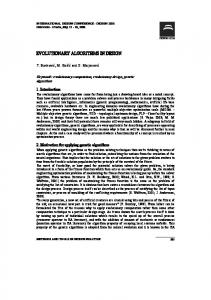
5 Discussion In a number of studies, the smoothness of the trajectory has been considered an important feature of a good solution in the optimization of bioprocesses, and new filtering or smoothing reproduction operators were proposed [18]. The proposed EA rewards smooth trajectories in the sense that its populations start with individuals that in average have a small number of points (around 10). The number only increases if the fitness function rewards a less smooth trajectory. As an example, in Figure 2 the feeding profile obtained (in the best run) for case study I by the new EA shows a quite smooth trajectory.

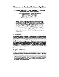
Figure 3: Convergence of the traditional EAs and the automatic interpolation (case study II). operators. The plain RCGA obtains a result of 32.41, while the alternatives with filtering operators obtain results in the range between 32.64 and 32.67. In case study I, the results are better than the ones obtained by using a gradient based algorithm, implemented by the MATLAB optimization toolbox function fmincon (version 2.1). The detailed results can be found in [15].

6 Conclusions and further work Figure 2: Feeding trajectory obtained by the EAs best run (case study I). Furthermore, this new representation easily allows the control of the smoothness of the trajectory by limiting the size of the individuals or favoring operators such as the shrink mutation. One important question to discuss is the capability of each of the algorithms to provide a good solution within limited CPU time constraints. The proposed approach does not impose an increase in the computational burden, when compared to the traditional EA. Furthermore, the proposed EA reaches good solutions faster than the traditional EAs. In Figure 3 it is shown a graph of the convergence of the two best traditional EAs and of the automatic interpolation EA for case study II. It is clear that the proposed EA achieves better solutions in less generations. A similar behavior can be observed in the other two case studies. Another issue that is important to discuss is the global quality of the results obtained by the different EAs. In fact, the values of the PIs obtained for case studies II and III are quite competitive with the ones previously published for the same problems. In case study II, the work reported in [8] obtains an average value of 20357.2, which is better than the results obtained in [4], using sequential quadratic programming. In case study III, the work reported in [19] uses several alternatives based on a Real Coded Genetic Algorithm (RCGA) combined with a number of specialized filtering

In this work a novel EA was proposed in order to optimize the feeding trajectory in fed-batch bioreactors. A new representation was suggested to encode the values of a variable over time. This representation contemplates the use of variable size chromosomes, where each gene consists of a pair time label (integer) - value (real number). A number of reproduction operators were adapted or built to work with this representation. It was shown that this new EA effectively optimizes the feeding trajectory, automatically handling interpolation/ discretization issues and producing good results in terms of the performance index and smooth profiles. Three distinct case studies were taken as benchmarks, with quite distinct features, namely when looking at the optimal feeding profiles. In previous work, real valued EAs were developed to simultaneously optimize the feeding trajectory, the initial conditions and the duration of a fermentation process (case study I). In the future, the new representation proposed here will be extended to handle the optimization of the initial values of the state variables and also to allow the optimization of the final time of the process. The quantitative model that serves as a base for the simulations done in this work is based on differential equations. Other types of models have been proposed in literature, namely Fuzzy Rules or Artificial Neural Networks [20][11]. The testing of the proposed EAs in these settings is desirable. Another area of future research is the consideration of on-line adaptation, being the model of the process updated

during the fermentation process, a task that can be also performed by EAs. In this case, the good computational performance of the proposed EAs are a benefit, if there is the need to re-optimize the feeding given a new model and values for the state variables measured on-line. Furthermore, a number of parameters in the proposed EA can be adjusted, namely the selection procedure (e.g. by considering stochastic universal sampling). Since the EA also makes use of several genetic operators, it would be interesting to study the adaptation of its probabilities along the evolution of tbe algorithm, following a strategy that was firstly proposed by Davis [6].

Acknowledgments The authors would like to acknowledge the support from the Portuguese Foundation of Science and Technology, under the project 54899/EIA/POSI/2004, partially funded by FEDER.

Bibliography [1] P. Angelov and R. Guthke. A Genetic-Algorithmbased Approach to Optimization of Bioprocesses Described by Fuzzy Rules. Bioprocess Engin., 16:299– 303, 1997. [2] J.R. Banga, C. Moles, and A. Alonso. Global Optimization of Bioprocesses using Stochastic and Hybrid Methods. In C.A. Floudas and P.M. Pardalos, editors, Frontiers in Global Optimization - Nonconvex Optimization and its Applications, volume 74, pages 45– 70. Kluwer Academic Publishers, 2003. [3] A.E. Bryson and Y.C. Ho. Applied Optimal Control - Optimization, Estimation and Control. Hemisphere Publication Company, New York, 1975.

[9] Z. Michalewicz. Genetic Algorithms + Data Structures = Evolution Programs. Springer-Verlag, USA, third edition, 1996. [10] H. Moriyama and K. Shimizu. On-line Optimization of Culture Temperature for Ethanol Fermentation Using a Genetic Algorithm. Journal Chemical Technology Biotechnology, 66:217–222, 1996. [11] J.G. Na, Y.K. Chang, B.H. Chung, and H.C. Lim. Adaptive Optimization of Fed-Batch Culture of Yeast by Using Genetic Algorithms. Bioprocess and Biosystems Engineering, 24:299–308, 2002. [12] S. Park and W.F. Ramirez. Optimal Production of Secreted Protein in Fed-batch Reactors. AIChE J, 34(9):1550–1558, 1988. [13] I. Rocha. Model-based strategies for computer-aided operation of recombinant E. coli fermentation. PhD thesis, Universidade do Minho, 2003. [14] I. Rocha and E.C. Ferreira. On-line Simultaneous Monitoring of Glucose and Acetate with FIA During High Cell Density Fermentation of Recombinant E. coli. Analytica Chimica Acta, 462(2):293–304, 2002. [15] I. Rocha and E.C. Ferreira. Optimisation Methods for Improving Fed-batch Cultivation of E. coli Producing Recombinant Proteins. In Proc. of the 10th Mediterranean Conference on Control and Optimization, Lisbon, 2002. [16] M. Rocha, P. Cortez, and J. Neves. Evolutionary Approaches to Neural Network Learning. In F. Pires and S. Abreu, editors, Progress in Artificial Intelligence, Proceedings of the EPIA’2003, LNAI 2902. Springer, 2003.

[4] C.T. Chen and C. Hwang. Optimal Control Computation for Differential-algebraic Process Systems with General Constraints. Chemical Engineering Communications, 97:9–26, 1990.

[17] M. Rocha, J. Neves, I. Rocha, and E. Ferreira. Evolutionary algorithms for optimal control in fed-batch fermentation processes. In G.Raidl et al., editor, Proceedings of the Workshop on Evolutionary Bioinformatics - EvoWorkshops 2004, LNCS 3005, pages pp.84–93. Springer, 2004.

[5] J.P. Chiou and F.S. Wang. Hybrid Method of Evolutionary Algorithms for Static and Dynamic Optimization Problems with Application to a Fed-batch Fermentation Process. Computers & Chemical Engineering, 23:1277–1291, 1999.

[18] J.A. Roubos, G. van Straten, and A.J. van Boxtel. An Evolutionary Strategy for Fed-batch Bioreactor Optimization: Concepts and Performance. Journal of Biotechnology, 67:173–187, 1999.

[6] L. Davis. Handbook of Genetic Algorithms. Van Nostrand Reinhold, 1991. [7] F. Herrera, M. Lozano, and J. Verdegay. Tackling Real-Coded Genetic Algorithms: Operators and Tools for Behavioral Analysis. Artif. Intel. Review, 12:265– 319, 1998. [8] V. Jayaraman, B. Kulkarni, K. Gupta, J. Rajesh, and H. Kusumaker. Dynamic Optimization of Fed-Batch Bioreactors Using the Ant Algorithm. Biotechnology Programming, 17:81–88, 2001.

[19] D. Sarkar and J. Modak. Genetic Algorithms with Filters for Optimal Control Problems in Fed-Batch Bioreactors. Bioprocess Biosystems Engineering, 26:295– 306, 2004. [20] A. Tholudur and W.F. Ramirez. Optimization of Fedbatch Bioreactors Using Neural Network Parameters. Biotechnology Progress, 12:302–309, 1996. [21] V. van Breusegem and G. Bastin. Optimal Control of Biomass Growth in a Mixed Culture. Biotechnology and Bioengineering, 35:349–355, 1990.