the antecedent conditions of fuzzy rules makes it a suitable ... approach. Rule-weight has often been used as a simple mechanism ..... Bangkok, Thailand., pp.
Proceedings of the World Congress on Engineering 2009 Vol I WCE 2009, July 1 - 3, 2009, London, U.K.
A New Rule-weight Learning Method based on Gradient Descent S.M. Fakhrahmad and M. Zolghadri Jahromi
Abstract— In this paper, we propose a simple and efficient method to construct an accurate fuzzy classification system. In order to optimize the generalization accuracy, we use ruleweight as a simple mechanism to tune the classifier and propose a new learning method to iteratively adjust the weight of fuzzy rules. The rule-weights in the proposed method are derived by solving the minimization problem through gradient descent. Through computer simulations on some data sets from UCI repository, the proposed scheme shows a uniformly good behavior and achieves results which are comparable or better than other fuzzy and non-fuzzy classification systems, proposed in the past. Index Terms— Fuzzy systems, Classification, Rule-weight, Distance, Generalization accuracy, Gradient Descent
I. INTRODUCTION Fuzzy rule-based systems have recently been used to solve classification problems. A Fuzzy Rule-Based Classification System (FRBCS) is a special case of fuzzy modeling where the output of the system is crisp and discrete. Different approaches used to design these classifiers can be grouped into two main categories: descriptive and accurate. In the descriptive approach, the emphasis is placed on the interpretability of the constructed classifier. In this approach, the classifier is usually represented by a compact set of short (i.e., with a few number of antecedent conditions) fuzzy rules. Using linguistic values to specify the antecedent conditions of fuzzy rules makes it a suitable tool for knowledge representation. However, the main objective in designing accurate FRBCSs is to maximize the generalization accuracy of the classifier. No attempt is made to improve the understandability of the classifier in this approach. Rule-weight has often been used as a simple mechanism to tune a FRBCS. Fuzzy rules of the following form are commonly used in these systems. Rule Rj: If x1 is Aj1 and … and xn is Ajn then class h with CFj (1) where, X=[x1, x2, …, xn] is the input feature vector, h ∈ [C1, C2 …, CM] is the label of the consequent class, Ajk is the fuzzy set associated to xk , CFj is the certainty grade (i.e. rule-weight) of rule Rj. S. M. Fakhrahmad is Faculty member in the department of computer engineering, Islamic Azad University of Shiraz, Iran; e-mail: mfakhrahmad@ cse.shirazu.ac.ir. M. Zolghadri Jahromi is Associate Professor in the department of computer science and engineering, Shiraz University, Iran; e-mail: zjahromi@ shirazu.ac.ir.
ISBN: 978-988-17012-5-1
Many heuristic [1, 2] and learning methods [3] have already been proposed to specify the weights of fuzzy rules in a FRBCS. The purpose of rule weighting is to use the information from the training data to improve the generalization ability of the classifier. In this paper, we propose a simple and efficient method of constructing accurate fuzzy classification systems. Using a specified number of triangular fuzzy sets to partition the domain interval of each feature, we propose a rule generation scheme that limits the number of generated fuzzy rules to the number of training examples. Each rule uses all features of the problem in the antecedent to specify a fuzzy subspace in feature space. We use rule weight as a simple mechanism to tune the constructed rule-base and propose an efficient rule-weight specification method. The rest of this paper is organized as follows. In Section 2, FRBCSs are briefly introduced. In Section 3, two different methods of rule-base construction is given. In Section 4, the proposed method of rule-weight learning is discussed. Experimental results are presented in Section 5. Finally, Section 6 concludes the paper. II. FUZZY RULE-BASED CLASSIFICATION SYSTEMS A FRBCS is composed of three main conceptual components: database, rule-base and reasoning method. The database describes the semantics of fuzzy sets associated to linguistic labels. Each rule in the rule-base specifies a subspace of pattern space using the fuzzy sets in the antecedent part of the rule. The reasoning method provides the mechanism to classify a pattern using the information from the rule-base and database. Different rule types have been used for pattern classification problems [4]. For an n-dimensional problem, suppose that a rule-base consisting of N fuzzy classification rules of form (1) is available. In order to classify an input pattern Xt = [xt1, xt2, …, xtn], the degree of compatibility of the pattern with each rule is calculated (i.e., using a T-norm to model the “and” connectives in the rule antecedent). In case of using the product as T-norm, the compatibility grade of rule Rj with the input pattern Xt can be calculated as: n
μ j (X t ) = ∏ μ A (x ti ) i =1
(2)
ji
In the case of using single winner reasoning method, the pattern is classified according to the consequent class of the winner rule Rw. With the rules of form (1), the winner rule is specified using:
w = arg max{μ j (X t )CFj , j = 1,..., N }
(3)
WCE 2009
Proceedings of the World Congress on Engineering 2009 Vol I WCE 2009, July 1 - 3, 2009, London, U.K.
Note that the classification of a pattern not covered by any rule in the rule-base is rejected. The classification of a pattern Xt is also rejected if two rules with different consequent classes have the same value of µ(Xt).CF in equation (2).
III. RULE-BASE CONSTRUCTION For an M-class problem in an n-dimensional feature space, assume that m labeled patterns Xp=[xp1, xp2, …, xpn], p=1, 2, …, m from M classes are given. A simple approach for generating fuzzy rules is to partition the feature space by specifying a number of fuzzy sets (i.e., k) on the domain interval of each input attribute. Some examples of this partitioning (using triangular membership functions) are shown in Fig. 1. Given a partitioning of pattern space, one approach is to consider all possible combinations of antecedents for generating the fuzzy rules. The selection of the consequent class for an antecedent combination (i.e. a fuzzy rule) can be easily expressed in terms of confidence of an association rule from the field of data mining [5]. A fuzzy classification rule can be viewed as an association rule of the form A j ⇒ class C j , where, Aj is a multi-dimensional fuzzy set representing the antecedent conditions and Cj is a class label. Confidence (denoted by C) of this fuzzy association rule is defined as [6]:
∑
C ( A j ⇒ class C j ) =
X p ∈ class C j
μ j (X p ) (4)
m
∑μ p =1
j
(X p )
Where, µj(Xp) is the compatibility grade of pattern Xp with the antecedent of the rule and m is the number of training patterns. The consequent class Cq of an antecedent combination Aj is specified by finding the class with maximum confidence. This can be expressed as:
q = arg max {C ( Aj ⇒ class h | h = 1, 2,..., M }
(5)
Note that, when the consequent class Cq can not be uniquely determined, the fuzzy rule is not generated. The problem with grid partitioning is that for an ndimensional problem, kn antecedent combinations should be considered. It is impractical to consider such a huge number of antecedent combinations when dealing with high dimensional problems. In this paper, we use two different solutions to tackle the above problem. We had introduced them in [7], [8], as two different methods for efficient rule generation in high dimensional problems. Our goal is to assess the effect of the new rule-weight learning method, proposed in this paper, on both of the systems. A. The 1st Approach to Rule Generation
The goal of this method is to propose a solution that enables us to generate fuzzy rules with any number of antecedents, i.e., there would be no restriction on the number of antecedents especially for high dimensional data sets (the problem which originates from the exponential growth of rule-base by increasing the number of features). For this purpose, we consider the well-known evaluation measure, Support as the primary factor for rule filtering. In equation (6), a simple definition for the fuzzy aspect of the Support measure is presented. s(Aj ⇒ Class h) = 1 ∑ m x p∈ Class h
μ A (x ) j
p
(6)
, where µj(Xp) is the compatibility degree of Xp with the antecedent part of the rule Rj, m is the number of training patterns and h is a class label. After determining a minimum support threshold (denoted by MinSupp), a set of 1dimensional rules (containing one antecedent), is generated. This set is then filtered by selecting only rules having a support value above the MinSupp. Combining the rules within this set in the next step, results in the set of 2dimensional candidate rules. The 1-dimensional rules which are pruned through the first step because of their bad supports, can not absolutely lead to 2-dimensional rules with good supports and thus there is no need to consider them. Another key point in combination of a pair of 1-dimensional rules is the conditions under which the rules can be combined: 1) The rules must not contain similar antecedents on their left-hand sides. 2) The consequent classes of the two rules must be identical. Similarly, the resulting rule set is filtered with respect to the MinSupp value. However, note that the rules being selected according to their higher support values are just candidate rules and may be rejected in the next step. The rule selection metric will be discussed later. In order to generate rules containing more than two antecedents, a similar procedure is followed. Generating 3dimensional rules is accomplished using the 1 and 2dimensional candidate rules. Any possible combination of the rules from these two sets, having the same consequent and not containing common antecedents would be a 3dimensional candidate rule. Of course, some principles are considered in order to avoid the time-consuming evaluation of some useless rules (which can not have high support values). Following the above process, it will also be possible to generate rules having 4 and more antecedents, for any data set having arbitrary number of features. Although the set of rules is pruned to some extent, in some cases the number of rules is still large. This problem gets more sensible as we increase the number of antecedents. In order to obtain a more concise data set, we divide the set of candidate rules into M distinct groups, according to their consequents (M is the number of classes). The rules in each group are sorted by an appropriate evaluation factor and the final rule-base is constructed by selecting p rules from each class, i.e., in total, M.p rules are selected. Many evaluation measures have already been proposed [9]. In this work, we use the measure proposed in [10] as the rule selection metric, which evaluates the rule A j ⇒ class C j through the following equation:
ISBN: 978-988-17012-5-1
WCE 2009
Proceedings of the World Congress on Engineering 2009 Vol I WCE 2009, July 1 - 3, 2009, London, U.K.
e (R j ) =
∑
X p ∈Class C j
μ A (x p ) − q
∑
X p ∉Class C j
μA (x p )
This method of rule generation is illustrated and discussed in more details in [7]. B. The 2nd Approach to Rule Generation Unlike the first approach, in this method, all of the generated rules are equi-length. Every rule's premise includes all the features of the dataset under investigation. The main idea in this method is to generate a fuzzy rule only if it has at least one training pattern in its decision area. Using fuzzy sets of Fig.1, to partition each attribute of a problem, a pattern is in the decision area of a rule only if each attribute value of the pattern has a membership greater than 0.5 in the corresponding antecedent condition of that rule.
For a specific problem, assume that the method of previous section is used to generate a set of N fuzzy rules. Initially, all rules are assumed to have a weight of one (i.e. CFk=1, k=1,2,...,N). In this section we propose an algorithm that assigns a weight in the interval [0,∞] to each rule. Our objective is to minimize the following index that represents the leave-one-out misclassification rate of the classifier:
1 w ≠ .μ ≠ (x ) J = ∑Step ( = = ) n x w .μ (x )
⎧1 if τ ≤ 1 Step (τ) = ⎪⎨ ⎪⎩0 if τ > 1
above
0.0
1.0
0.0
1.0
1.0
0.0 0.0
0.0 1.0
formulas,
the
pairs
(w , μ =
=
(x ) )
1.0
1.0
derivative of J with respect to weights (i.e., w and w ). For this purpose, we approximate the step function by the sigmoid function:
0.0
≠
=
0.0
and
(w , μ (x ) ) represent the weights and the compatibility grades associated to the rules of the same-class and the different-class that are most compatible with pattern x, respectively. In order to minimize J using gradient descent, we need the ≠
0.0
(8)
Where, the step function is defined as:
In
1.0
1.0
IV. THE PROPOSED METHOD OF RULE WEIGHTING (GDW1)
(7)
q
Fig. 1. Different partitioning of each feature axis
As an example, for a 2-feature problem with four fuzzy sets on each feature, the decision areas of 16 fuzzy rules are shown in Fig. 2. Note that, although the covering areas of different rules are overlapped, their decision areas are not. As we only generate a rule if it has at least one training pattern in its decision area, the number of rules generated will be at most equal to the number of training patterns. Making use of this key issue, the time complexity of the rule generation process in high dimensional problems is reduced to O(m), where m is the number of training patterns (i.e., compared to O(kn)).
Φ (τ ) =
1 (1 + e β (1−τ ) )
≠
(9)
Replacing the step function in (8), we have:
1 w ≠ .μ ≠ (x ) J = ∑ Φ( = = ) n x w .μ (x )
(10)
To simplify (10), we define r(x) as:
w ≠ .μ ≠ (x ) r (x ) = = = w .μ (x ) Using this, equation (10) can be re-written as:
J =
Fig. 2. Decision areas of 16 fuzzy rules.
1 ∑ Φ(r ( x )) n x
To derive the gradient descent update equations, we need to use Φ'(τ), which is given as:
Φ′( τ) =
1
ISBN: 978-988-17012-5-1
(11)
∂Φ (βe β(1−τ) ) = ∂τ (1 + e β(1−τ) ) 2
(12)
Gradient-Descent-based Weighting
WCE 2009
Proceedings of the World Congress on Engineering 2009 Vol I WCE 2009, July 1 - 3, 2009, London, U.K.
Φ'(τ) is a function whose maximum value occurs in τ =1 and vanishes for |τ −1|>>0. This function approaches the Dirac delta function for large values of β. For small values of β, it is approximately constant in a wide range of its domain. Regarding the mentioned equations, the following gradient descent equation is obtained to be used for updating the rule weights.
∂J ∂J ∂Φ ∂r * * = = ∂w ∂Φ ∂r ∂w = − w ≠ .μ ≠ (x ) = ∑ Φ′(r (x ))* = 2 = (w ) .μ (x ) x
(13)
Similarly,
∂J ∂J ∂Φ ∂r = * * ≠ ∂w ∂Φ ∂r ∂w ≠ μ ≠ (x ) = ∑ Φ′(r (x ))* = = w .μ (x ) x
(14)
To adjust the weights of the rules, the algorithm starts by visiting each training example (i.e., x) and updates the weights of two rules (i.e. the same-class and different-class rules that are most compatible with pattern x). The optimization process can terminate after a specified number of passes over the training data or when no significant improvement of the performance index J was observed over previous pass. The weight update law can be expressed as: w ≠ .μ ≠ (x ) = = w new = w old + η . ∑ Φ′(r (x )) * = 2 = (15) (w ) .μ (x ) x ≠ ≠ w new = w old − η.
∑ Φ′(r (x )) * x
μ ≠ (x ) w = .μ = (x )
(16)
where η is a small positive real number that represents the learning factor of the algorithm. The rule-weight learning algorithm is given in Fig. 3. Algorithm GDW(D, R, W, β, η, ε) { // D: training data set; R,W: initial rule-base and weights; // β: sigmoid slope; η: learning factor; ε: a small constant number λ' = ∞; λ = J(R,W); P' = P; W' = W while (|λ' - λ|> ε) { λ' = λ for each x in D { rule= = NearestRule_SameClass(R,W,x) rule≠ = NearestRule_DiffClass(R,W,x) i = index(rule=) k = index(rule≠) z1 = Φ'(r(x), β) * (W[k] / (W[i])2) * ((μk(x)) / ( μi(x))) ; z2 = Φ'(r(x), β) * ((μk(x)) / ( W[i]*μi(x))) ; W'[i] = W'[i] + η * z1 W'[k] = W'[k] - η * z2 } P = P'; W = W'; λ = J(R,W) } return W }
One of the parameters needed by the algorithm is υ. It can take just a fixed value for i or may vary among different rules using some heuristics; for example, it may be proportional to the no. of right-class patterns existing in the decision area of a rule. Moreover, for smoother (but slower) convergence, we had better decrease this factor value along the successive iterations of the algorithm's loop. In general, the value of this factor may have a significant impact on the learning speed but, as long as it is not too large, it should not have an important influence on the learning results. A generally suitable value for the learn step factor to be used for any data can not be found since it depends on the nature and characteristics of the training data. The effect of the update equation in the learning algorithm is obvious. The rule-weight learning mechanism is much related to the Reward-And-Punishment approach used in some well-known methods in the literature, such as LVQ1, LVQ2 [11, 12] and DSM [13]. In an iterative manner, each training pattern, x, rewards its nearest rule that classifies it correctly (by increasing the associated weight). Meanwhile, it punishes another rule, having the maximum compatibility to x, which misclassifies it (by decreasing the associated weight). During this learning process, the decision areas of the rules covering many compatible patterns and few incompatible ones grow more significantly. 5. Experimental results To measure the effectiveness of the proposed ruleweighting scheme in improving the generalization ability of the constructed rule-base, we used the data sets of Table I available from UCI ML repository. To construct an initial rule-base for a specific data set, each feature was first normalized to interval [0,1]. For rule-base construction, we followed both of the methods given in section 3, in turn. When applying the second method, we used five triangular fuzzy sets to partition the domain interval of each feature. To assess the generalization ability of various schemes, we used ten-fold cross validation scheme [14]. For a given training subset, a rule-base was generated using one the methods of Section 3 and the method of Section 4 was then used to specify the weight of each fuzzy rule. Five trials of ten-fold cross validation were performed to calculate the average error-rate of the classifier on test data. First of all, in order to evaluate the effect of the weighting method on the generalization ability, the accuracy of each of the two classifiers presented in Section 3 was monitored before and after rule-weigh specification. In Fig. 6, we report on generalization error-rate of the rule-base before and after rule weighting for various data sets. In Table II, we report on ten-fold generalization ability of the system using both methods of rule generation, in turn. GDW(1) and GDW(2) stand for the proposed scheme when using the first and the second approaches of rule generation, respectively. The proposed scheme is compared with different weighting methods on fuzzy classifiers defined by Ishibuchi in [15]. The results are also compared with two other fuzzy classifier given in [3], [8], respectively. The first classifier uses a method of rule weight learning based on ROC analysis, while the second follows a heuristic weighting method. The competitive results for these fuzzy rule-based classifiers are given in Table II. In all schemes, the rule selection is performed using the single winner reasoning method.
Fig. 3. Rule-weight Learning algorithm.
ISBN: 978-988-17012-5-1
WCE 2009
Proceedings of the World Congress on Engineering 2009 Vol I WCE 2009, July 1 - 3, 2009, London, U.K.
50 Without rule-weights
45
With rule-weights
Error rates (%)
40 35 30 25 20 15 10 5 0 Iris
Wine
Pim a
Bupa
Thyroid
Glass
Sonar
Datasets
(a) 45
Without rule-weights
40
With rule-weights
Error rates (%)
35 30 25 20 15 10 5 0 Iris
Wine
Pima
Bupa
Thyroid
Glass
Sonar
Datasets
(b) Fig. 6. The effect of rule-weight learning scheme on reducing the error rates of the classifier for benchmark datasets: (a) using the 1st method of rule generation, (b) using the 2nd method of rule generation
ISBN: 978-988-17012-5-1
WCE 2009
Proceedings of the World Congress on Engineering 2009 Vol I WCE 2009, July 1 - 3, 2009, London, U.K. Table I. Some statistics of the data sets used in our computer simulations.
Data set
Number of attributes
Number of patterns
Number of Classes
Iris Wine Pima Australian German Heart Bupa Landsat Balance Scale Thyroid Voting Liver Glass Letter Sonar Vehicle
4 13 8 14 20 13 6 36 4 5 16 7 9 6 60 18
150 178 768 690 1000 270 345 6435 625 215 435 345 214 20000 208 946
3 3 2 2 2 2 2 6 3 3 2 2 6 2 2 4
Table II. Classification Error rates of the new classifier (GDW) using two different methods of rule generation ((1), (2)), in comparison with other fuzzy rule-based classifiers: Non-weighted fuzzy classifier, Ishibuchi weighting methods (4 methods) and the heuristic weighting method of [8] Error Rates (%) Data sets
No. Weight
Iris Wine Pima Bupa Thyroid Glass Sonar
5.0 6.1 27.8 39.0 8.5 35.0 11.2
Ishibuchi (1) 4.2 6.7 26.5 38.8 6.1 44.4 10.8
(2) 4.4 5.6 27.8 38.8 6.3 40.6 10.6
(3) 4.6 8.4 26.5 38.4 5.8 40.2 10.8
[9]
REFERENCES [1] [2] [3] [4] [5] [6] [7]
[8]
E. Mansoori, M. Zolghadri Jahromi and S.D. Katebi, A weighting function for improving fuzzy classification systems performance Fuzzy Sets and Systems 158 (5) (2007), 583-591. M. Zolghadri Jahromi and E. Mansoori, Weighting fuzzy classification rules using receiver operating characteristics (ROC) analysis, Information Sciences 177 (11) (2007), 2296-2307. M. Zolghadri Jahromi and M. Taheri, A proposed method for learning rule weights in fuzzy rule-based classification systems, Fuzzy Sets and Systems, (2007). O. Cordon, M. J. del Jesus, F. Herrera, A proposal on reasoning methods in fuzzy rule- based classification systems, International Journal of Approximate Reasoning 20 (1999) 21-45. R. Agrawal, R. Srikant, Fast algorithms for mining association rules, in: Proc. 20th International Conference on Very large Databases, 1994, pp. 487-499. H. Ishibuchi, T. Yamamoto, Fuzzy rule selection by multi-objective genetic local search algorithms and rule evaluation measures in data mining, Fuzzy Sets and Systems 141 (1) (2004) 59-88. S.M. Fakhrahmad, A. Zare and M. Zolghadri Jahromi, "Constructing Accurate Fuzzy Rule-based Classification Systems Using Apriori Principles and Rule-weighting" The 8th International Conference on Intelligent Data Engineering and Automated Learning (IDEAL'07), Birmingham, U.K , pp. 457-462, December 2007,. S.M. Fakhrahmad and M. Zolghadri Jahromi, "Constructing Accurate Fuzzy Classification Systems: A New Approach Using Weighted Fuzzy Rules", 4th International Conference (IEEE) on Computer Graphics, Imaging and Visualization, (CGIV07), Bangkok, Thailand., pp. 408-413, 15-17 August 2007.
ISBN: 978-988-17012-5-1
[10] [11] [12]
[13] [14] [15] [16] [17] [18]
(4) 4.2 8.4 26.3 39 6.7 41.1 11.0
GDW
ROC-based method
Heuristic method
(1)
(2)
4.9 3.7 24.6 34.5 4.2 38.2 25.8
3.6 5.1 24.3 37.8 4.1 33.3 4.1
2.9 4.7 21.6 34.3 4.2 29.9 13.7
1.7 5.0 21.4 37.3 3.8 31.4 8.0
H. Ishibuchi, T. Yamamoto, Comparison of heuristic criteria for fuzzy rule selection in classification problems, Fuzzy Optimization and Decision Making 3 (2) (2004) 119-139. A. Gonzalez, R. Perez, SLAVE: A genetic learning system based on an iterative approach, IEEE Trans. on Fuzzy Systems 7 (2) (1999) 176-191 T. Kohonen, The self-organizing map, in: Proceedings of the IEEE, vol. 78, 1990, pp. 1464–1480. T. Kohonen, G. Barna, R. Chrisley, Statistical pattern recognition with neural networks: benchmarking studies, in: IEEE International Conference on Neural Networks, vol. 1, San Diego, 1988, pp. 61– 68. S. Geva, J. Sitte, Adaptive nearest neighbor pattern classification, IEEE Trans. Neural Networks 2 (2) (1991) 318–322. C. Goutte, Note on free lunches and cross-validation, Neural Computation, 9 (1997) 1211-1215. H. Ishibuchi, T. Yamamoto, Rule Weight Specification in Fuzzy Rule-Based Classification systems, IEEE Transaction on Fuzzy Systems 13 (4) (2005) 428-435. Elomaa, T. and J. Rousu. “General and efficient multisplitting of numerical Attributes,” machine Learning 36 (1999), 201-244. V. Vapnik, Statistical Learning Theory,Wiley-Interscience, NewYork, 1998. Roberto Paredes, Enrique Vidal, Learning prototypes and distances: A prototype reduction technique based on nearest neighbor error minimization, Pattern Recognition 39 (2006) 180 – 188.
WCE 2009