research field, especially in client-server databases and dis- ... DBMS that supports SQL queries. Suppose that a ... null (this is true for this example), it has to be sent to the server. ... query. The best case is achieved when a semantic region.
A Semantic Caching Method Based on Linear Constraints Yoshiharu Ishikawa Hiroyuki Kitagawa Institute of Information Sciences and Electronics University of Tsukuba Tsukuba, Ibaraki, 305-8573 Japan {ishikawa,kitagawa}@is.tsukuba.ac.jp
Abstract Because performance is a crucial issue in database systems, data caching techniques have been studied in database research field, especially in client-server databases and distributed databases. Recently, the idea of semantic caching has been proposed. The approach uses semantic information to describe cached data items so that it tries to exploit not only temporal locality but also semantic locality to improve query response time. In this paper, we propose linear constraint-based semantic caching as a new approach to semantic caching. Based on the idea of constraint databases, we describe the semantic information about the cached relational tuples as compact constraint tuples. The main focus in this paper is the representation method of cache information and the cache examination algorithm.
1. Introduction Data caching has been investigated in various fields of database research such as client-server databases [5, 18], data warehouses [6], and distributed and heterogeneous databases [1]. In client-server environments, the method can be described as follows. 1. When a query is issued, the client cache manager checks its own cache. If part of the requested data items already exists in the cache, the client can start its local query processing. 2. To obtain the remaining part of data items, the client sends a request to the server. 3. After the client finishes its local query processing, it stores the obtained new data items into its cache. Since the cache space is bounded, it must use a cache replacement policy to decide which data items to replace when the cache is full.
As described above, we can improve query response time in client systems using caching techniques. Caching is effective when temporal locality exists in the access patterns between a query and its preceding queries; this condition holds in many cases, especially in client-server environments in which each client has its own access pattern. A caching technique, however, has an overhead to maintain cache contents to be up-to-date. Therefore, a client cache manager has a responsibility to decide which data items to be retained using a cache replacement policy. In the traditional caching approach, cached data items (typically physical pages or tuples) were maintained based on temporal locality. Recently, some researchers have proposed the semantic caching approach, which manages cached data items using semantic locality along with temporal locality [5, 16]. In this approach, a client maintains semantic descriptions of cached data items, instead of maintaining a list of physical pages or tuple identifiers. Query processing is performed using the semantic descriptions to determine what data items are available in the local cache and what data items are to be obtained from the server. The use of semantic information encourages the effective use of cached data items. To describe semantic information, Dar et al used rectlinear spatial regions [5]: cached data items are associated with rectangles in the semantic space. The predicate caching method, proposed by Keller and Basu, used predicates to describe cache contents [16]. In the method, predicates are used only to accumulate the reference count for each cached item and not interpreted—they are regarded as black boxes. In this paper, we extend the approach of [5] and describe semantic information using linear arithmetic constraints. We adopt the idea of constraint databases [8, 15] to represent cached tuples; the semantic information is compactly represented as a set of constraint tuples. The rest of the paper is organized as follows. Section 2 presents a motivating example of semantic caching. In Section 3, we mention to the related work. Section 4 introduces a constraint database model to describe cached relational
tuples. Section 5 presents the cache examination and replacement algorithms. Finally, in Section 6, we give the discussion and conclude the paper.
cache-info tid constraint tuple t1 ( displacement ≥ 1500 ) ∧ ( price ≤ 8000 )
2. A Motivating Example Let us assume that the server contains the following relation: UsedCar(name, maker, year, displacement, price, tax, ...)
In this example, we assume that the server is a relational DBMS that supports SQL queries. Suppose that a user wants to select used cars with displacement more than or equal to 1,500 cc and less than 8,000 dollars in price. The user will submit the following query to the client system: Q1: SELECT name, year FROM UsedCar WHERE displacement >= 1500 AND price = 1500 AND price = 1200 AND price + tax 0 dc price : price > 0 dctax : tax ≥ 0 A domain constraint is given as an (in)equality constraint, typically given by the database designer, and represents the range of possible values that the attribute (variable) can take. Although we can use part of the cached base tuples to process query Q2, we still need to submit a request to obtain the remaining tuples. Such a query is called a reminder query and given by ¬ q1 ∧ q2 . If the reminder query is not null (this is true for this example), it has to be sent to the server. Finally, the client updates the table cache-info as shown in Fig. 3.
cache-info tid constraint tuple t1 ( displacement ≥ 1500) ∧ ( price ≤ 8000) t2 ( displacement ≥ 1200) ∧ ( price + tax ≤ 10000)
time T1 T2
Figure 3. Updated cache information
3. Related Work 3.1. Semantic caching The semantic caching approach [5, 16] uses semantic descriptions to represent the client cache contents. Dar et al. [5] used a semantic region to represent the cached data items obtained by a query. A semantic region is defined as a rectlinear spatial region and compactly represented by a simple conjunctive form such as q = ( salary > 50000) ∧ ( age ≤ 30 ). The main difference between their approach and our proposal is that their semantic regions are restricted to rectangle shapes. Although the rectlinear region-based representation has an advantage of low calculation and maintenance costs, it cannot represent arithmetic constraints expressed by a linear combination of attributes. On the other hand, if we use the terminology of computational geometry [7], a semantic region in our context is a convex polyhedron defined by the intersection of half-spaces specified by linear arithmetic constraints. In this sense, our approach includes the rectangle region-based semantic caching approach. Linear arithmetic constraints are considered to be becoming more important because the emergence of several new database application domains (e.g., OLAP, GIS, and scientific databases) requires more efficient complex query handling facilities [9]. In the semantic region-based approach [5], a client cache manager determines whether cached data items can be used to process the given query. For its decision, it examines the semantic regions of cached items to find overlaps with the query. The best case is achieved when a semantic region or a combination of semantic regions completely covers the semantic region of the query so that the client can process the query without contacting the server. In this case, the client only issues a probe query to retrieve data items from the local cache. In other cases, the cache does not contain some or all of the required data items; the client cache manager, therefore, has to submit a reminder query to request remaining data items in addition to a probe query. Note that the query processing can be interleaved—the client query processor can start its query processing using the current cache content without waiting the completion of the reminder query. One additional advantage of the semantic region-based caching is its compact representation of re-
minder queries. As another approach of semantic caching, Keller and Basu proposed the predicate caching method [16]. In this method, client cache contents are described by predicates that are contained in the preceding queries issued to the client systems. In contrast to our approach and [5], the semantics of a predicate is not used explicitly. A predicate is considered to be a black box and used to calculate reference counts for each cached data item. We can find other approaches to semantic caching. Adalı et al proposed the intelligent cache method for distributed mediated environments [1]. It provides sophisticated use of cache mechanism using domain knowledge and additional information. Their approach was directly applied to Web caching applications by Chidlovskii et al [4].
3.2. Materialized view The methodology of data caching has close relationship with that of materialized view management [14]. The ADMS project by Roussopoulos et al [17, 18, 19] is especially related to our research. Roughly speaking, their approach is to cache (materialize) intermediate query results and access paths, obtained while processing the incoming queries, dynamically into the local cache. The cached materialized views and access paths are reused by the subsequent queries based on the notion of subsumption, the containment relationship between queries. However, the judgment of subsumption relationship becomes complicated if we consider queries generated by arbitrary combination of relational operators. In contrast to their approach, our approach, like [5], uses a set of base tuples as a caching unit so that the judgment load is alleviated. Moreover, the semantic region-based caching uses overlap relationship between queries to decide the availability of cached items. Therefore, it has more flexibility than subsumption-based (containment-based) approaches.
3.3. Constraint databases A constraint database is a kind of database incorporating the notion of constraints directly into the data model to model infinite information with finite representation using arithmetic constraints [3, 8, 11, 15]. The aim of constraint database model is to represent spatial or temporal information directly based on constraints. We can find many research attempts on constraint databases such as discussion of the expressive power of some constraint data model and spatial object representation scheme based on a constraint data model. Constraints can be incorporated into database models at different levels [15]; a constraint data model is determined by specifying a base data model (e.g., relational data model
and object-oriented data model), a database language (e.g., relational calculus and datalog), and a constraint domain (e.g., dense order, linear arithmetic, and polynomials). The constraint data model used in this paper is based on the relational data model, and its constraint domain is linear arithmetic constraints over rational numbers Q. The reasons to use linear arithmetic constraints are: 1) it has a sufficient expressive power to represent constraints that occur in practical situations, and 2) the computational complexity to handle linear arithmetic constraints is moderate one [11]. As shown in the next section, we have not included a database language in the constraint data model because it is sufficient to describe our semantic cache method without the help of a data manipulation language.
4. Data Model
numeric domain (e.g., rational numbers Q and real numbers R). The constraints we consider in this paper belong to the first-order language L = {≤ , +} ∪ Q. This class of language has a good tradeoff between the query processing power and its computational complexity [10, 13]. In addition to the term constraint domain, we use the term uninterpreted domain to specify an attribute domain that cannot be associated to numeric values. We assume that only constraints regarding ’=’ and ’≠’ can be specified over an uninterpreted domain. A constraint over rational numbers Q has the following form: a 1 x1 + … + a p x p θ a 0 , (1) where xi is a variable, ai is an integer constant (1 ≤ i ≤ p), and θ satisfies θ ∈ {= , ≠, < , ≤ , > , ≥} .
In this section, we briefly define a simple constraint data model to describe cache contents. Our model of constraint databases is mainly based on those of Grumbach et al [11] and Kanellakis et al. [15].
4.1. Basic definition A constraint k-tuple (or generalized k-tuple), in variables x1 , …, xk that range over a set D, is a finite conjunction Φ1 ∧ … ∧ ΦN , where each Φi (1 ≤ i ≤ N) is a constraint. If the arity (or the number of dimension) k is clear from the context, we omit k, and use the term constraint tuple. There are a lot of kinds of constraint tuples depending on the kinds of constraints used. In all case, equality constraints and inequality constraints among individual variables and constants are allowed. For example, ( x = 3 ∧ y ≠ 2 ) represents a constraint 2-tuple. We can observe that a relational tuple (e.g., ( 3, 2 )) can be expressed by using equality constraints as above. Therefore, we can interpret any relational tuples as constraint tuples. A constraint relation of arity k (a generalized relation of arity k) over a set D is a finite set r = {ϕ1 , …, ϕM }, where each ϕi (1 ≤ i ≤ M) is a constraint k-tuple in the same variables x1 , …, xk . The formula corresponding to a constraint relation r is the disjunction ϕ1 ∨ … ∨ ϕM . It is in disjunctive normal form (DNF) of constraints, which uses at most k variables ranging over set D. Each constraint relation describes a finite set of arity k tuples (or points in k-dimensional space Dk ) and represents a possibly infinite set of arity k tuples. A constraint database is a finite set of constraint relations.
4.2. Linear constraints A constraint in a constraint data model is usually represented by a first-order language and interpreted over some
(2)
The term ai xi is an abbreviation of xi + … + xi (ai times). In this paper, we use linear arithmetic constraints along with the constraint data model defined in subsection 4.1 as the data model to describe the semantic information in a client cache. A constraint relation defined as above sometimes called a linear constraint relation.
4.3. Orthographic partitioning The computational complexity of processing constraints highly depends on the class of constraint domain and the number of variables (i.e., the number of dimensions) contained in constraints. It is problematic especially for large databases that contain many attributes. To cope with this problem, Grumbach et al put restrictions on linear constraint relations and gave an upper bound of the query complexity [12]. Although their context is quite different from ours (since we do not need the full expressive power of the linear constraint data model), their idea can be applicable to reduce the processing cost in our context. The idea is based on the idea of dependent variables: if two variables appear in the same linear constraint, we call these variables dependent; otherwise they are independent. For example, in the example in Section 2, variables (attributes) price and tax are dependent because they have appeared in the same constraint. On the other hand, displacement and price are independent because they usually do not appear in the same constraint formula. Based on this idea, we can group variables into some orthographic partitions in terms of dependency. In the example of Section 2, we can obtain two orthographic partitions: op1 = {displacement} and op2 = {price, tax}. If we incorporate the notions of dependency and orthographic partition, the cost of constraint manipulation does not depend on the total number of variables—it depends on the partition
with the largest number of variables. The number of variables of the largest partition is called orthographic dimension. Orthographic dimension is an important factor to estimate upper bounds of operations over constraint databases. If we incorporate the idea of orthographic partition, we can represent cache-info relation shown in Fig. 3 as in Fig. 4. Namely, each orthographic partition is stored independently in cache-info relation. This representation will reduce the computation cost and introduce flexibility to incorporate indexes for the efficient query processing (see Section 7).
cache-info id op1 q1 displacement ≥ 1500 q2 displacement ≥ 1200
op2 price ≤ 8000 price + tax ≤ 8000
time T1 T2
Figure 4. Partitioned representation
5. Using Cache Information In this section, we show how to use the cache information represented by a constraint relation to generate the probe query and the reminder query for a given query.
5.1. Cache examination algorithm As described in Section 2, when a client receives a query q, it examines the constraint tuples in the cache-info relation to generate the probe query pq and the reminder query rq. Figure 5 shows the algorithm for the examination of cache information. The algorithm is naive in the sense that it examines all the constraint tuples in cache-info ; we will present some ideas to improve the algorithm in Section 7. We have to make some definitions to explain the algorithm. Let the number of constraint tuples in cache-info relation be n and the number of orthographic partitions be k. Then assume that the given conjunctive query has a general form q = q1 ∧ q2 ∧ … ∧ qk , where each qi corresponds to ith orthographic partition opi . If q has no corresponding condition for opi , let qi : = T . The symbol ’T ’ means the Boolean truth value; the false value is defined as F = ¬ T . For example, the constraint ( displacement ≥ 1500) ∧ ( price ≤ 8000) , appeared in Section 2, has q1 = ( displacement ≥ 1500 ) and q2 = ( price ≤ 8000) for the orthographic partitions op1 = {displacement} and op2 = {price, tax}, and the constraint ( price ≤ 8000) ∧ ( price + tax ≤ 10000)
has q1 = T and q2 = ( price ≤ 8000) ∧ ( price + tax ≤ 10000). In the algorithm, we assume that qi ≠ T for i = 1, …, l and qi = T for i = l + 1, …, k to simplify the presentation. 1. 2. 3. 4. 5. 6. 7. 8. 9. 10. 11. 12. 13. 14. 15. 16. 17. 18.
for i : = 1 to n { // for each constraint tuple ti ci, j : = constraint part of ti for op j ( j = 1,…, k); for j : = 1 to l { pqi, j : = compute-overlap ( q j , ci, j ); if (pqi, j ≡ F) { // cannot use tuple ti for q pqi : = F; goto line 1; // check next tuple ti + 1 } } pqi : = pqi, 1 ∧ … ∧ pqi, l ; … ∧ ci, k ; pq+ i : = pqi ∧ ci, l + 1 ∧ } pq : = pq1 ∨ … ∨ pqn ; // probe query … ∨ pq+ pq+ : = pq+ n ; // augmented probe query 1 ∨ if (pq ≡ q) rq : = F; // no need of reminder query else rq : = q ∧ ¬ pq+ ; // reminder query
Figure 5. Naive cache examination algorithm Now we look into the algorithm. The algorithm examines each constraint tuple ti (i = 1,…, n) to generate the probe query pq and the reminder query rq. We assume that the tuple ti has the form ti = ci, 1 ∧ ci, 2 ∧ … ∧ ci, k ; each ci, j corresponds to the orthogonal partition op j ( j = 1,…, k) and takes the value ci, j = T when ti does not contain the corresponding condition for op j . At lines 3–9, the following process is repeated for each orthographic partition. At line 4, the compute-overlap function (described in subsection 5.3) is called and the overlapped region of two constraints is calculated. The function takes two conjunctive constraints as arguments and computes their overlap (namely, the conjunction of two constraints), then returns a new conjunctive constraint as a result. If two constraints do not have an intersection, the function returns F. The probe query for ti , denoted by pqi , is constructed by AND-ing pqi, j for j = 1 to l (line 10). Similarly, pq+ i is constructed by augmenting pqi with ci, l + 1 ,…, ci, k . At lines 13 and 14, the probe queries pq and pq+ are constructed by OR-ing pqi ’s and pq+ i ’s, respectively (i = 1,…, n). As shown in the example below, these two forms of probe queries generate the same result when they are evaluated over the local cache, but pq is much simpler than pq+ and preferable. The query pq+ is necessary only to generate the reminder query rq : = q ∧ ¬ pq+ (line 18). At the final step of the algorithm, it checks whether pq ≡ q or not. If it is true, the client can process the query q without submitting a reminder query since the probe query pq retrieves all the tuples which q wants. Therefore, the reminder query is set
to rq : = F. As an example, let Fig. 6 be the current contents of cache-info (we have omitted time field to simplify the presentation) and the given query be q = ( 1400 ≤ displacement ≤ 1600) ∧ ( price ≤ 7000) . We have q1 = ( 1400 ≤ displacement ≤ 1600 ), q2 = ( price ≤ 7000 ), k = 3, and l = 2. Using the above algorithm, we get pq = pq1 ∨ pq2 , where pq1 = ( 1500 ≤ displacement ≤ 1600 ) ∧ ( price ≤ 7000 ) and pq2 = ( 1400 ≤ displacement ≤ 1600 ) ∧ ( price ≤ 7000) ∧ ( price + tax ≤ 8000 ). The augmented probe query is given as + rq+ = rq+ ∨ rq+ 1 2 , where rq1 = rq1 ∧ ( year ≤ 1998 ) and + rq2 = rq2 ∧ ( 1997 ≤ year ≤ 1999). The reminder query is constructed as rq = q ∧ ¬ pq+ .
cache-info id op1 t1 displacement ≥ 1500 t2 displacement ≥ 1200
op2 price ≤ 8000
op3 year ≤ 1998
price + tax ≤ 8000
1997 ≤ year ≤ 1999
Figure 6. An example of cache information
5.2. Local query processing When a query q is given, the client begins its query processing. The client query processing steps are shown below. 1. The client calculates the probe query pq and the reminder query rq based on the cache examination algorithm. 2. If pq ≠ F, the client evaluates pq to retrieve tuples from its local cache. 3. If rq ≠ F, the client sends rq to the server to obtain the remaining tuples then continues its query processing. 4. After the query processing is finished, the client stores all the obtained tuples into its local cache (if the cache area is exhausted, the client triggers the cache replacement procedure—see Section 7). 5. Finally, the client adds a new tuple into cache-info and updates other statistical information. For example, it increments the reference counter for each tuple accessed (and cached) by the query q. In the above algorithm, we have not considered domain constraints to simplify the presentation. It is easy to incorporate domain constraints into the above algorithm.
5.3. Overlap computation In subsection 5.1, we did not mention how to calculate compute-overlap. In this subsection, we explain its calculation method. Before we describe the method, two requirements for compute-overlap are shown: 1. It calculates the overlap of two given conjunctive constraints: if the overlap is empty, the function returns the false value F. 2. It is desirable to delete redundant constraints from the given constraints. For example, it must reduce a constraint ( age > 30 ) ∧ ( age ≤ 50 ) ∧ ( age > 40 ) to ( age > 40 ) ∧ ( age ≤ 50 ). For simple constraints (such as 1D or 2-D rectlinear constraints), we can easily detect redundant constraints. However, it is not obvious to detect redundant constraints for linear arithmetic constraints. To calculate the overlap region of two constraints, and to detect redundant constraints, we extend the idea found in linear programming literature [20]. Note that the procedure given below is rather general one; we can choose algorithms that are more efficient by observing specific conditions satisfied in each situation. For example, if the number of dimension is one or two, we can use more efficient computation methods using the techniques found in computational geometry [7]. First, we normalize the given constraints: 1. Decompose the constraints into constraints in the normal form (Eq. (1)). For example, 0 < x ≤ 100 is transformed into x > 0 and x ≤ 100. 2. If a constraint has the form a1 x1 + … + a p x p = a0 , transform it, for example, into the form x1 = a11 ( … ), for example, and then delete x1 from all of the constraints. Namely, we can reduce the number of variables (dimensions). 3. If the constraint has the form a1 x1 + … + a p x p > a0 , rewrite it to a1 x1 + … + a p x p ≥ a0 . The same transformation is applied to the case of ’ m): a11 x1 + … + a1n xn a21 x1 + … + a2n xn .. . am1 x1 + … + amn xn
= =
b1 b2 .. and xi ≥ 0 .
( i = 1,…, n )
= bm
We can transform the above formulas into matrix and vector notations: Ax x
= b ≥ 0,
(4) (5)
where x ≥ 0 represents that every element xi of x satisfies xi ≥ 0. 5. All of the basic feasible solutions are calculated. This can be attained by solving Am xm = b at most ( mn ) times [20], where Am and xm are an m × m matrix and an m-d vector induced from A and x, respectively. 6. If there is no basic feasible solution, we can conclude that the conjunction of two given constraints is not satisfied (namely, two constraints do not have an overlap). 7. If there are one or more basic feasible solutions, the overlap between two constraints exists. From these basic feasible solutions, we can derive a set of nonredundant constraints easily. As a result, we can obtain a conjunctive constraint c = c1 ∧ … ∧ cr that satisfies Eq. (4) and Eq. (5). 8. Constraints according to ’≠’ are processed as follows. Let a non-redundant constraint obtained in step 7 be c = c1 ∧ … ∧ cs . For each constraint a1 x1 + … + a p x p ≠ a0 , call the function compute-overlap ( c, a1 x1 + … + a p x p = a0 ). If the result is F, do nothing since the additional constraint a1 x1 + … + a px p ≠ a0 does not interfere with c. Otherwise, replace c with c : = c ∧ ( a1 x1 + … + a p x p ≠ a0 ). 9. We have to compensate the effect of step 3 where ’>’ and ’ a0 was replaced into cb ≡ a1 x1 + … + a p x p ≥ a0 in step 3. If we can find cb in the set of non-redundant constraints {c1 , …, cr } obtained in step 7, replace cb with the original constraint ca . If we cannot find cb in {c1 , …, cr }, do nothing. If the overlap exists, compute-overlap returns the final conjunctive constraint c = c1 ∧ … ∧ cr as a result.
6. Cache Replacement Algorithm Since the cache area in the client system is bounded, we usually need to replace old cached items with incoming new data items. For the cache replacement problem, we must clarify 1) the selection method of a victim (the target of replacement), and 2) the cache replacement algorithm. To select a victim, the client cache manager has to consider several factors such as the freshness and the access frequency of the cached items and uses a cache replacement policy (e.g., LRU) to make a decision. It depends on the situation which kind of cache management mechanism is appropriate. Therefore, here we do not specify the actual cache management method and simply assume that the select-victim function, which selects an appropriate victim, is available. The cache replacement algorithm is shown in Fig. 7. We denote the constraint tuple specified as a victim by tv . In the algorithm, a simple reference count-based method is used. For the selected victim (constraint tuple) tv , the corresponding base tuples V = {bt1 , …, btn } are retrieved from the cache and then the reference count for each bti is decremented by 1. Finally, the cache manager deletes all of the base tuples with reference count 0. 1. 2. 3. 4. 5. 6. 7. 8. 9. 10.
tv : = select-victim ( ); let qv be the constraint corresponding to tv ; submit query qv to the local cache; let V = {bt1 , …, btn } be the query result; for i : = 1 to n { re f count ( bti ) : = re f count ( bti ) − 1; if (re f count ( bti ) ≡ 0) delete bti from the cache; } delete tv from cache-info;
Figure 7. Cache replacement algorithm To make this replacement algorithm work correctly, the cache manager has to maintain the reference count for each cached base tuple. Therefore, when a base tuple is accessed by a probe query or a reminder query, the cache manager has to increment its reference count correctly.
7. Discussion and Conclusion The cache examination algorithm described in subsection 5.1 scans all the constraint tuples in cache-info relation. This causes a critical problem when cache-info relation is large. One of the solutions to this problem is the use of indexes. For constraint databases, there have been several proposals of indexing techniques [2]. Since indexing methods for constraint databases depend on the number of variables (dimensions), the actual constraint maintenance
cost depends on orthographic partitions that determine the actual number of dimensions to be considered. Therefore, the selection method of indexes also depends on them. If the number of variables (dimensions) of an orthographic partition is one or two, efficient indexing methods for constraint databases are available [2]. If the number of dimensions is more than two, two approaches exists: 1) Project each constraint on one or two dimensions, and then use above-mentioned indexing methods, 2) Extract minimum bounding boxes (MBBs) from each constraint then use them as spatial indexes. Such a spatial index can be used in the filtering step to select the candidates of constraint tuples that may satisfy the condition. To reduce the computational overhead of the naive algorithm shown in subsection 5.1, we can also use indexes and approximations. When a query q is given, we first search the candidate constraint tuples using indexes. Next, we can use approximation-based comparisons (e.g., using MBBs to approximate constraints) to filter out unnecessary constraint tuples. Then we start the exact comparison by the algorithm shown in this paper. In this paper, we have proposed a new semantic caching approach based on linear arithmetic constraints. We adopted the idea of constraint databases to represent cached base tuples by compact constraint tuples. This paper mainly focused on the cache examination algorithm to utilize cached information, the method to calculate the overlap of two semantic regions, and the cache replacement algorithm. The remaining issues are the cache examination algorithm incorporating approximation, the use of indexes for the efficient cache management, and development of efficient cache replacement policies and their comparisons.
Acknowledgments This work was partially supported by the Grant-in-Aid for Scientific Research from the Ministry of Education, Science, Sports and Culture of Japan.
References [1] S. Adalı, K. S. Candan, Y. Papakonstantinou, and V. S. Subrahmanian. Query caching and optimization in distributed mediator systems. In Proc. of ACM SIGMOD, pages 137– 148, Montreal, Quebec, Canada, June 1996. [2] E. Bertino, B. C. Ooi, R. Sacks-Davis, K.-L. Tan, J. Zobel, B. Shidlovsky, and B. Catania. Indexing Techniques for Advanced Database Systems. Kluwer Academic, 1997. [3] A. Brodsky and Y. Kornatzky. The LyriC language: Querying constraint objects. In Proc. ACm SIGMOD, pages 35–46, San Jose, CA, May 1995. [4] B. Chidlovskii, C. Roncancio, and M.-L. Schneider. Semantic cache mechanism for heterogeneous web querying. In Proc. 8th Intl. WWW Conf., Toronto, Canada, May 1998.
[5] S. Dar, M. J. Franklin, B. T. J´osson, D. Srivastava, and M. Tan. Semantic data caching and replacement. In Proc. of VLDB, pages 330–341, Mumbai, India, Sept. 1996. [6] P. M. Deshpande, K. Ramasamy, A. Shukla, and J. F. Naughton. Caching multidimensional queries using chunks. In Proc. of ACM SIGMOD, pages 259–270, Seattle, Washington, USA, June 1998. [7] H. Edelsbrunner. Algorithms in Combinatorial Geometry. Springer-Verlag, 1987. [8] V. Gaede and M. Wallace. An informal introduction to constraint database systems. In V. Gaede, A. Brodsky, O. G¨unther, D. Srivastava, V. Vianu, and M. Wallace, editors, Constraint Databases and Applications, volume 1191 of LNCS, pages 7–52. Springer-Verlag, 1997. [9] J. Goldstein, R. Ramakrishnan, U. Shaft, and J.-B. Yu. Processing queries by linear constraints. In Proc. of ACM PODS, pages 257–267, Tucson, Arizona, May 1997. [10] S. Grumbach and G. M. Kuper. Tractable recursion over geometric data. In Proc. Intl. Conf. on Constraint Programming (CP97), volume 1330 of LNCS, pages 450–462, Linz, Austria, Oct.-Nov. 1997. [11] S. Grumbach, P. Rigaux, and L. Segoufin. The DEDALE system for complex spatial queries. In Proc. of ACM SIGMOD, pages 213–224, Seattle, Washington, USA, June 1998. [12] S. Grumbach, P. Rigaux, and L. Segoufin. On the orthographic dimension of constraint databases. In C. Beeri and P. Buneman, editors, Proc. of 7th ICDT, volume 1540 of LNCS, pages 199–216, Jerusalem, Israel, Jan. 1999. [13] S. Grumbach, J. Su, and C. Tollu. Linear constraint query languages: Expressive power and complexity. In D. Leivant, editor, Workshop on Logic and Computational Complexity, LNCS. Springer-Verlag, Indianapolis, Oct. 1994. [14] A. Gupta and I. S. Mumick, editors. Materialized Views. MIT Press, 1999. [15] P. C. Kanellakis, G. M. Kuper, and P. Z. Revesz. Constraint query languages. J. Comput. Syst. Sci., 51(1):26–52, Aug. 1995. [16] A. M. Keller and J. Basu. A predicate-based caching scheme for client-server database architectures. VLDB Journal, 5(1):35–47, Jan. 1996. [17] N. Roussopoulos. An incremental access method for ViewCache: Concept, algorithms, and cost analysis. ACM Trans. Database Syst., 16(3):535–563, Sept. 1991. [18] N. Roussopoulos, C. M. Chen, S. Kelly, A. Delis, and Y. Papakonstantinou. The ADMS project: Views “R” us. IEEE Data Engineering Bulletin, 18(2):19–28, June 1995. [19] N. Roussopoulos, N. Economou, and A. Stamenas. ADMS: A testbed for incremental access methods. IEEE TKDE, 5(5):762–774, Oct. 1993. [20] A. Schrijver. Theory of Linear and Integer Programming. John Wiley and Sons, New York, 1986.