A New Theoretical Approach: A Model Construct for Fault ...
Recommend Documents
Crystal growth theories and catalytic reaction mechanisms share common fundamentals on ...... Crystal Growth and Design 1, 225â229. Kubota, N., Mullin, J.W., ...
ABSTRACT. The shrinkage or swelling of coal as a result of gas desorption or adsorption is a well-accepted phenomenon. Its impact on permeability changes ...
Appropriately Targeted Reading Comprehension Source Texts. Kathleen M. ... evaluated via machine learning techniques (e.g., Naïve Bayes, k-Nearest ...
of the communication buffers as well as concurrent DMA transfer. This novel communication model is applied in our rapid prototyping environment for optimizing ...
ARTISTIC PARODY: A THEORETICAL. CONSTRUCT. SHERRI L. BURR*. In
Living Color, the television show, produces a parody called. Am I Black or White?
1 ...
plate and a layer of metal foam or honeycomb as core. ... Figure 1: In-structure shock of surface structure with metal foam cladding subjected to close range blast.
GRIDTS: A New Approach for Fault-Tolerant Scheduling in Grid Computing. Fábio Favarim ..... some of the fields jobId and taskId, which identify the job and the ...
Jan 12, 2016 - Equation (6) represents a circle with the center at A and passing through F: ... Equation (9) sets the straight line passing through Points B and E:.
snapshot in an asynchronous distributed system (as the In- ternet) has a classical .... the tuple space state stays valid according to the semantics of application when ..... dling the ticket, transaction 1 puts one job tuple describing the job, and
of monitoring programmes and delivering cost-effective services, and shortening bureaucratic .... a single window inform
where multicast trees are constructed in MPLS networks ... warding scheme that extend routing with respect to packet forwarding and path .... Traceroutre experiments result from one source at ... routers. We also obtained results from a set of tracer
A Theoretical Construct for South-South Cooperation. Sachin Chaturvedi ...... Email: [email protected], Website: http:
Dec 1, 2010 - Toxicogenomics using microarray technology has recently been applied to 2,4DNT and other military compounds to understand its molecular ...
shame from failing to achieve the American dream that he commits suicide by the final act of the play. In Wil- liam Shakespeare's Macbeth, Lady Macbeth is so.
To evaluate the software tool UNISIM in. To evaluate the software ... Semicontinuous High grade A. 02 CENT_B ... Semicontinuous Low grade. Characteristics of ...
Center for Research on Information Technology and Organizations (CRITO). 3200 Berkeley ... Alladi Venkatesh, University of California, Irvine. Franco Nicosia ...
processes requires advanced supervision and fault ... applications in factory, home and automotive areas, ... Advanced methods of supervision, fault detection.
former is applicable for measuring strain in a unique direction only, whereas ..... [20] Wood J R, Zhao Q, Frogley M D, Meurs E R, Prins A D,. Peijs T, Dunstan D J ...
Nov 30, 2017 - [6] Samir Khuller, Manish Purohit, and Kanthi K. Sarpatwar. âAnalyzing the optimal neighborhood: Algorithms for budgeted and partial.
This research addresses the issue of hospital stockpile levels in preparing ... of its supplies) to another hospital only when it is not responding to the pandemic.
u.wr~riq. II' this nc\r vccior spiicc rcprcscntcd by a unit coiisisrs 01' aril), ;I single signature, thcn thc fault case associarcd wirli hiit signature can hc isolated.
Comunicación y educación en el Perú (1993); La edad de la pantalla. ... A educomunicação é um campo de estudo fundado por correntes teóricas ... crítico para a compreensão das interações entre indivíduos e os media, a atenção às práticas ..... Educom
Summary. Darwinian paradigm of biological evolution is based on the independence of genetic variations from selection which occurs afterwards. However ...
dition is proposed for the existence of the minimal âManhattanâ routes in presence .... take either west or south direction, making a Manhattan routing impossible.
A New Theoretical Approach: A Model Construct for Fault ...
Sep 6, 2017 - of the repair action determining the efficacy of troubleshooting. In this paper, we propose a new theoretical algorithm to construct a model for ...
Hindawi Mobile Information Systems Volume 2017, Article ID 9038634, 16 pages https://doi.org/10.1155/2017/9038634
1. Introduction Cloud computing refers to flexible, self-service, and networkaccessible computing resource pools that can be allocated to meet demand, allowing thousands of virtual machines (VMs) to be used even by small organizations. As the scale of cloud deployments continues to grow, the necessity for scalable monitoring tools that support the unique requirements of cloud computing is of greater priority [1]. Endowing clouds with fault-troubleshooting abilities for the management of the reduction, existing complexity, and continued development of the complexity of a utility cloud [2] presents a difficult but obviously interesting solution. Troubleshooting for faults in the cloud remains relatively unexplored so that there has been no universally accepted tool chain or systems for the purpose. In the presented work fault detection is defined as a problem of classifying the time instances during runtime in which cloud computing is having anomalies and faults [3]. A useful algorithm in which the problem needs to be addressed
must contain the following: (a) high detection and rates with few false alarms; (b) an independently supervised technique due to insufficient a priori knowledge regarding standard or anomalous behavior, or circumstances; (c) an autonomic methodology so that the increase in cloud scaling includes personnel costs. Additionally, a cloud is typically used by multiple tenants and multiple VMs may be colocated on the same host server [4]. Because resources such as CPU usage, memory usage, and network overhead are not virtualized, there exists a complex dynamism between the VMs, which have to share resources. The increased complexity is hugely problematic in terms of troubleshooting [5]. However, it is unsuitable for environments with dynamic changes, is susceptible to high false-alarm rates, and is expected to perform poorly in the context of large-scale cloud computing [6]. Current monitoring tools are service tools, such as Nagios and Ganglia [7, 8] which are designed with greater functionality to obtain low-level metrics including the CPU, disk, memory, and I/O, but not designed to service
2 monitoring for dynamic cloud environments. Current apparatus are founded on threshold methods, which in industry monitoring commodities are more frequently employed. First, upper and lower bounds are created for all of the metrics. The threshold values come from the knowledge of performance along with predictions rooted in the historical data analysis from the long-term. Violation of the threshold limit by any of the observed metrics triggers an alarm of anomaly. Therefore, in this paper we propose a new theoretical approach for constructing the steps of a faulttroubleshooting model. The model combines a Na¨ıve-Bayes classifier (NBC) with a multivalued decision diagram (MDD) and influence diagram (ID) to structure and manage fault troubleshooting. An NBC is a simple probabilistic classifier algorithm based on the application of a Bayesian network (BN) with independence assumptions between predictors [9, 10]. The NBC is a modeling technique based on probability, which is the most acceptable for knowledge-based diagnostic systems which are knowledge-based. Ultimately this allows for the modeling and reasoning regarding uncertainty. An NBC and an ID were developed in the artificial intelligence community as principled formalisms for reasoning and representing under uncertainty in intelligent systems [11]. Therefore, this technique is ideally suited for the diagnosing in real-time world complication where uncertain incomplete datasets exist [12]; this method offers an appropriate mechanism for diagnosing complicated virtualization systems in the cloud. The major advantage of using a BN is its ability to represent and hence allow knowledge to be understood. A BN comprises two parts: qualitative knowledge through its network structure and quantitative knowledge through its parameters. Whereas expert knowledge from practitioners is mostly qualitative, it can be used directly for building the structure of a BN [13]. In addition, data mining algorithms can encode both qualitative and quantitative knowledge and are able to encode both forms of knowledge simultaneously in a BN. Therefore, BNs can bridge the gap between different types of knowledge and serve to unify all knowledge availability into a single form of representation [14]; therefore, an NBC is suitable for producing probability estimates rather than predictions. These estimates allow predictions to be ranked and their expected costs to be minimized. The NBC still provides a high degree of accuracy and speed when applied to large datasets [5]. A MDD is a generalization of the binary decision diagrams (BDD), which have been used to model static multistate systems for reliability and availability analysis. MDDs are one of the effective mathematical methods for the representation of multiple-valued logic (MVL) functions of large dimensions. They have recently been adapted for the reliability analysis of fault tolerant systems [15, 16]. The MDD can quickly categorize the degree of the risk of consequences according to the symptoms [17]. Specifically in relation to prior work, an NBC and a MDD have been widely used in many research projects and applications that require dependability, self-diagnosis, and monitoring abilities, especially in terms of fault diagnosis and monitoring systems [18]. Zhai et al. [5] proposed a method for the analysis of the multistate system (MSS) structure function by a BN
Mobile Information Systems and a Multistate System (MSS), which is an effective approach for the analysis and estimation of high-dimensional functions in MVL. Sharma et al. [6] developed CloudPD as the first innovative end-to-end fault management system capable of detecting, diagnosing, classifying, and suggesting remediation actions for virtualized cloud-based anomalies. Wang et al. [19] proposed EbAT, a system for anomaly identification in data centers that analyzes system metric distributions rather than individual metric thresholds. Smith et al. [20] proposed an availability model, which combines a highlevel fault tree model with a number of lower level Markov models of a blade server system (IBM BladeCenter). Xu et al. [21] proposed an approach based on BNs for error diagnosis. However, a comprehensive analysis indicates that these researchers who work in different research areas use Bayes’ theorem only for reasoning and for calculating the fault probability with threshold-based methods and other techniques for the detection of faults/anomalies, in which the tuning for sensitivity must be far-reaching in order to prevent an unacceptable number of false positives. Furthermore, the drawback of an extremely high number of false alarms is that it simply induces monitoring of individual metrics rather than monitoring metric combinations, which is more desirable. Thus, in contrast to previous research and contributions, this paper addresses fault troubleshooting in cloud computing. The objective of this work is to monitor collections, develop classifiers, and analyze attributions of metrics rather than individual metric thresholds by extending the diagnosis of faults into troubleshooting while multiple measurements of decisions are still considered including priority, fault probability, risk or severity, and duration of the construction steps for fault detection and repair actions. The contribution of this paper is the following: it proposes a new theoretical approach algorithm to construct the steps of a model for fault troubleshooting by combining NBC with MDD and an ID to structure and manage fault troubleshooting on cloud anomaly detection. The theoretical approach takes into account multiple measurements (criteria), such as the priority, fault probability, risk, and duration of the repair when making high priority decisions about repair actions. The NBC is used to determine the fault probability based on the use of a Na¨ıve-Bayes probabilistic model for fault diagnosis, whereas MDD and ID are used to subsequently combine the impact of the four measures and compute the utility value with the priority of the troubleshooting steps for each action to determine which fault is selected for repair. The decision for recovery repair is determined by the utility coefficient and the priority of the action for each repair. The case-study used in this work is the failure of a host server to start up. The theoretical proposition ensures that the most sensible action is carried out during the procedure of troubleshooting and generates the highest efficacy and cost-saving fault repair through three construction steps: (I) determining the network parameters which indicates the probability dependency relationship among all of the nodes; (II) evaluating the structure of the network topology; (III) assessing the probability of the fault being propagated, as shown in Figure 1.
Mobile Information Systems
3
Workflow Weights of criteria
OpenStack Measuring & monitoring devices
Data preprocessing
MDD
Utility value of fault (type, size, location)
NBC Repair
Host server
Ganglia metrics
Data Testing filtering dataset Network parameters
Training dataset Network topology structure
Probability propagation
Figure 1: Overview of fault-troubleshooting workflow.
The rest of the paper is organized as follows. Section 2 describes the fault-troubleshooting analysis based on MDD, determination of the action set, and the measurements criteria. In Section 3 we introduce the concepts of the NBC and ID models. Section 4 focuses on modeling uncertainty using the proposed approach and presents our ongoing work toward developing a framework based on NBC and its extension an ID network topology and phase of parameters process. Section 5 explains probability propagation for the NBC model. Section 6 explains the process of the troubleshooting decision. Section 7 explains the experimental setup for a single data center. Section 8 presents the method implementation, evaluation results, and a comparison with current troubleshooting methods. Finally, conclusions and future work are presented in Section 9.
2. Fault-Troubleshooting Analysis Based on MDD A troubleshooting process aims to perform, detect, and fix faults with high efficiency and with low risk. The success of each fix is ascertained by its likelihood of failure, risk, duration, and priority. The MDD is able to rapidly categorize the degree of the risk of faults according to the symptoms [11]. MDD investigation is a procedure covering the proposal of the complication to the execution of the ultimate action. The most important notions for the application of troubleshooting for faulty applications are given in Table 1. 2.1. Ascertainment of Action Groups and Measurements Specifications. There are four categories of causes of start-up failure in a cloud system: host server, host operating system, virtual machine monitor (VMM) [22], and VMs, as shown in Figure 2. In this paper, the failure of the host server to start up is used as a case-study to show the strategy of the method. Troubleshooting for faults of the procedure is separated into two steps: the first step is to ascertain the fault group that needs to be troubleshot, and for step two which part should be troubleshot needs to be determined. The set of actions is deterministic for each of the steps. In step one, a host server start-up failure can be the result of six
Table 1: Key notions for troubleshooting of faulty applications. Questions of decision
Determine the faulty components that should be repaired in each diagnostic stage
Objectives of decision
Determine and repair faults successfully
Maker of decision Measurement (criteria)
The categories for the set of actions
Troubleshooter with the highest priority Probability fault of component Duration Severity/risk of each repair action occurring Priority services The set of pairs of categories/elements (actions sets for which each process is deterministic)
types of failure as shown in Figure 2, CPU utilization (CPUutilization fault), memory (memory-leaks-fault), I/O storage (throughput-fault), network (bandwidth-fault), and other factors such as power/cooling failures; thus, the actions set in the first step includes the network, CPU, memory, storage, power, and cooling which is in need of repair. Thus, if a repair action of the CPU utilization is selected in the first step, step two will be used to select a set of actions to repair host-CPUusage, VM-CPU-usage, and VM-CPU-Read-Time errors. As mentioned before, to perform a troubleshooting decision, troubleshooters must examine the fault probability of the fault’s component and also the risk, duration, and priority required to repair the component faults. Four evaluation measurements criteria are determined: (1) probability of component failure; (2) duration; (3) risk; and (4) priority. Fault probability indicates the likelihood of fault components causing the failure of the host server to start up. Duration is defined as the time in minutes to complete the repair fault action. Risk is defined as the degree of risk (normal, minor, and serious) of creating additional new faults and making the troubleshooter aware of the safety issue during the repair action. Priority is the priority level service of the repair actions. Of the four quantification criteria,
4
Mobile Information Systems
Cooling
Power
Others
Memory usage
Host-
VM-CPU
VM-CPU-
CPU-usage
-usage
-Read-Time
Memory
Network
CPU
Bandwidth
Throughput
I/O storage
Host
Host server fault NBC model
VMM Host OS
System VMs
Figure 2: NBC availability model for a cloud system.
the likelihood of the fault being uncertain and the NBC diagnostic model can be used to determine such likelihood. The other three are confirmed for a particular action and are able to be inferred from expert understanding that had been accumulated over a period of time through investigation and time-consuming analysis. 2.2. Determine the Weights of Measurements. MDD assesses the effect of many measurements by computing the value of a utility in which each criterion has a specific measurement weight. The ranking method and pair-wise comparison method have been used in dictating the measurement weights. For this paper, the ranking method uses a criterion according to the importance that has been concluded to be believable by the decision makers and thus accordingly determines the weights [23]. The following formula is used for computing the weights: 𝑊𝑐 =
𝑛 − 𝑟𝑐 + 1 , ∑𝑛𝑥=1 (𝑛 − 𝑟𝑥 + 1)
(1)
where 𝑊𝑐 is the weight of measurement; 𝑐, 𝑛 are the decision criteria numbers; and 𝑟𝑐 is the measurement criterion in the status of hierarchical importance of 𝑐. Based on the domain expert’s opinion, the order of importance for each measurement is explained as follows:
Table 2: A sample weight of each of the measurement criteria. Criteria Weight
Fault probability 0.4
Risk 0.1
Priority 0.2
Duration 0.3
As seen in Table 2, a sample weight of each measurement is calculated by the ranking method.
3. Determining Fault Probability Using NBC and ID 3.1. The Na¨ıve-Bayes Probabilistic Model. A Na¨ıve-Bayes classifier [24] is a function that maps input feature vectors 𝑋 = {𝑥1 , . . . , 𝑥𝑛 }, 𝑛 ≥ 1, to output class labels 𝐶 = {𝑐1 , . . . , 𝑐𝑛 }, where 𝑋 is the feature space. Abstractly, the probability model for a Bayes classifier is a conditional model (𝐶 | 𝑥1 , . . . , 𝑥𝑛 ), which is the so-called posterior probability distribution [25]. Applying Bayes’ rule, the posterior can be expressed as
(1) Fault probability: first (2) Severity/risk: second (3) Priority: third (4) Duration: fourth.
where 𝑃(𝐶𝑖 /𝑋) is the posterior probability of the class (target) given predictor (attribute); 𝑃(𝐶𝑖 ) is the prior probability of the class; 𝑃(𝑋| 𝐶𝑖 ) is the likelihood probability of the given class; 𝑃(𝑋) is the prior probability of the predictor (evidence).
Mobile Information Systems
5
The simplest classification rule is used to assign an observed feature vector 𝑋 to the class with the maximum posterior probability.
Because ∑𝑛𝑖=1 𝑃(𝑋 | 𝑐𝑖 )𝑃(𝑐𝑖 ) is independent of 𝑐𝑖 and does not influence the arg max operator, classif y(𝑋) can be written as classif y (𝑋) = arg max (𝑋 | 𝑐𝑖 ) 𝑃 (𝑐𝑖 ) . 𝑐𝑖
(4)
This is known as the maximum a posteriori probability (MAP) decision rule [26]. The BN model that was established for fault diagnosis contains three aspects of work [27]: (1) Determine the network parameters to indicate the probability dependency relationship between all nodes; (2) Determine the network topology structure; (3) Probability propagation: this is to calculate the probability of each node given the evidence. In this paper, the purpose of building an NBC model is to determine the most likely cause of a fault, given a fault symptom, that is, to compute the end possibilities for the cause of the fault given the evidence [28]. The end possibility is calculated using the joint probability calculator. To further simplify this calculation, the conditional independence is determined by NBC to make some assumptions. Any node is independent of unlinked nodes and is dependent on its parent node. Thus, for any node 𝐶𝑖 , which belongs to a group of nodes, {𝐶1 , 𝐶2 , . . . , 𝐶𝑛 }, if there is a clear node 𝜋(𝐶𝑖 ) ⊆ {𝐶1 , 𝐶2 , . . . , 𝐶𝑛 }, 𝐶𝑖 will be conditionally independent of all other nodes except for that of 𝜋(𝐶𝑖 ). Conditional independent terms, according to the definition, are 𝑃(
𝐶𝑖 𝐶𝑖 ) = 𝑃( ). 𝐶1 , 𝐶2 , . . . , 𝐶𝑛 𝜋 (𝐶𝑖 )
(5)
Figure 3 is an example of the NBC model with the content arrangement of three layers with a four-node connection {𝑐1 , 𝑐2 , 𝑐3 , 𝑐4 }. According to (2), the posterior conditional probability can be obtained by 𝑃 (𝐶2 = True, 𝐶4 = True) 𝐶 = True 𝑃( 2 , )= 𝐶4 = True 𝑃 (𝐶4 = True)
(6)
where 𝑃(𝐶2 = True, 𝐶4 = True) and 𝑃(𝐶4 = True) are called marginal probability and can be calculated from 𝑃 (𝐶2 = True, 𝐶4 = True) = ∑ 𝑃 (𝐶2 = True, 𝐶1 , 𝐶3 , 𝐶4 = Ture) , 𝑐1 ,𝑐3
where 𝑃(𝐶2 = True, 𝐶1 , 𝐶3 , 𝐶4 = Ture) and 𝑃(𝐶1 , 𝐶2 , 𝐶3 , 𝐶4 = True) involve calculation of the joint probability. The joint probability 𝑃(𝐶1 , 𝐶2 , 𝐶3 , 𝐶4 ) can be calculated according to the definition of the chain rule and joint probability, from 4
3.2. The Influence Diagrams Model. Influence diagrams (ID) [29] for solving decision problems extend BN with two additional types of nodes, utility nodes and decision nodes. A utility node is a random variable whose value is the utility of the outcome [30]. Nodes for the random variables in the BN are called chance nodes in the ID. A decision node defines the action alternatives considered by the user. A decision node is connected to those chance nodes whose probability distributions are directly affected by the decision. A utility node is a random variable whose value is the utility of the outcome. Like other random variables, a utility node holds a table of utility values for all value configurations of its parent nodes [31]. In an ID, let 𝐴 = {𝑎1 , 𝑎2 , . . . , 𝑎𝑛 } be a set of mutually exclusive actions and 𝐻 the set of determining variables. A utility table 𝑈(𝐴, 𝐻) is needed for yielding the utility for each configuration of action and determining variable in order to assess the actions in 𝐴. The problem is solved by calculating the action that maximizes the expected utility: 𝐸𝑈 (𝑎𝑖 ) = ∑𝑈 (𝑎𝑖 ) 𝑝 (𝐻 | 𝑎𝑖 ) , 𝐻
(9)
where 𝐸𝑈(𝑎𝑖 ) represents the expected utility of action 𝑎𝑖 ; 𝑝(𝐻 | 𝑎𝑖 ) is the conditional probability of variables ℎ𝑖 , where 𝐻, given action 𝑎𝑖 , is executed. This conditional probability is calculated from the conditional probability table (CPT) while traversing the BN of these variables. Figure 4 represents an example of an ID of a CPU and a decision to detect a CPU-utilization fault. Prediction and CPU are chance nodes containing probabilistic information about the CPU and prediction. Satisfaction is a utility or value node. CPU utilization is a decision node. The objective is to maximize expected satisfaction by appropriately selecting values of CPU utilization for each possible prediction. The values of satisfaction for each combination of CPU utilization
6
Mobile Information Systems
CPU Prediction
Prediction
Host-CPU
VM-CPU
VM-CPU
-usage
-usage
-Read-Time
Normal
0.60
0.30
0.10
Fault
0.40
0.70
0.90
CPU
CPU Host-CPU-usage
0.60
VM-CPU-usage
0.30
VM-CPU-Read-Time
0.10
CPU
Sat.
Normal
Host-CPU-usage
9
Normal
VM-CPU-usage
2
Normal
VM-CPU-Read-Time
3
Fault
Host-CPU-usage
5
Fault
VM-CPU-usage
−4
CPU utilization
CPU utilization
Satisfaction
Fault
VM-CPU-Read-Time 10
Figure 4: Example of an influence diagram.
Cooling
Power
Memory usage
Host-CPU -usage
VM-CPU -usage
VM-CPU read-time
Bandwidth
Throughput
Network
I/O storage
Is fault?
Others
Memory
CPU
Host server state
Priority
System
Decision
Figure 5: NBC for host server start-up failure.
and CPU are also given. The evaluation of the algorithm of an ID is performed using the following procedure [31]: (1) Set the evidence variables for the current state. (2) For each possible value of the decision node, set the decision node to that value. (3) Calculate the posterior probabilities for the parent nodes of the utility node using a standard probabilistic inference algorithm. (4) Calculate the resulting utility function for the action and return the action with the highest utility.
4. Determination of NBC Network Topology In this section, we focus on modeling uncertainty using the proposed approach and present our ongoing work toward developing a framework based on NBC and ID models. 4.1. The Topology of the NBC Combined with an ID Model. As shown in Figure 5, start-up failure of the host server may have its roots in six groups of faults which include CPU utilization [32], memory usage, I/O storage, network overhead, and power and cooling failure [20]. Each group has some specific reasons as shown in Table 3. Using GeNle [33] the topology of the NBC combined with an ID model was created in accordance with the causes of the
Mobile Information Systems
7 Table 3: Fault reasons for the start-up failure of a host server.
Fault category
CPU utilization
Fault causes % CPU time used by host CPU during normal sampling period (host-CPU-usage) % CPU time during which the CPU of the VM was actively using the physical CPU (VM-CPU-usage) % CPU time during which the CPU of the VM was ready but could not get scheduled to run on the physical CPU (VM-CPU-Ready-Time)
Measurement level
VM, host
Memory
% of used memory (memory usage)
VM, host
Network
% of network usage (bandwidth)
VM, host
I/O storage
% of disk usage (throughput)
Host
Others
Cooling and power
Host
Table 4: Sample parameters dataset of CPU utilization (testing/training). Time-monitoring 12:02:00 AM 12:07:00 AM 12:12:00 AM 12:17:00 AM 12:22:00 AM 12:27:00 AM 12:32:00 AM 12:37:00 AM .. .
fault of the host server start-up failure, as shown in Figure 5. The model has eight chance nodes (conditions) for the root nodes pointing to the fault root causes (attribute values), which are shown in the yellow circles, five intermediate nodes pointing to the fault category (observed attributes), which are shown as green circles, a symptom node (predict) shown as an orange circle, one node indicating the priority drawn as a white circle, one decision node (Is fault?) drawn as a white rectangle, and the utility (decision) nodes drawn as the final white shape. As seen in Figure 3, each node in the graph is associated with a set of local (conditional) probabilities expressing the influence of the values of the nodes’ predecessors (parents) on the probabilities of the values of this node itself (e.g., Pr(𝑋𝑖 /𝑝(𝑋𝑖 )), (2)). These probabilities form the quantitative knowledge input into the NBC network. An important property of the network is (conditional) independence. The lack of a directed link between two variables from the CPUutilization node and host-CPU-usage node are independent, conditional on some subset 𝜑 of other variables in the model. For example, if no path existed between the CPU-utilization node and host-CPU-usage then 𝜑 will be empty. 4.2. Normal Distribution. Numerical data [34] need to be transformed to their categorical counterparts (binning) before constructing their frequency tables. Other options we
have are to use the distribution of the numerical variables to obtain a good estimate of the frequency. A normal probability distribution is defined by two parameters, 𝜇 and 𝜎. Besides 𝜇 and 𝜎, the normal probability density function (PDF) 𝑓(𝑥) also depends on the constants 𝑒 and 𝜋 [35]. The normal distribution is especially important as a sampling distribution for estimation and hypothesis testing. 4.3. Determination of Network Parameters. Parameters were taken from large monitoring engines (metric-collection) to obtain the metrics of interest (numerical predictors or attributes). Additional details are provided in Section 8, for example, for the Virtual Machine Manager (VMM) [36] hypervisor (testing dataset) and historical data (training dataset). Sample parameters of CPU utilization (testing/training dataset) are provided in Table 4. The metrics of the VMs and host server were collected by running the VMs on the Xen (hypervisor) [37, 38], which was installed on the host server in combination with preprocessing (reported in Table 3) using Ganglia metrics software. Because these metrics exist in the form of numerical data, the numerical variables had to be transformed into their categorical counterparts (binning) before constructing their frequency table to use them as input for the network topology structure [39]. Therefore, as shown in Figure 6, the preprocessing step consists of four steps to translate continuous
8
Mobile Information Systems Example parameters test data VMCPU%
A sample of the dataset probability using NBC model
M-event creations
Faultstate 3
M-event
Vector-value
M-E-t1
⟨1, 1, 1⟩
M-E-t2
⟨1, 1, 2⟩
M-E-t3
⟨4, 3, 3⟩
A sample of the dataset used for creating classification
Figure 6: Explanation of the method of the proposed approach and a sample of tables from the dataset.
percentage utilization into interval probability values and generate monitoring vectors of events (𝑀-events) by using the method proposed in [19]. We adopted this method with a filtering dataset to remove and process the outlier data and noise by using Extended Kalman Filter (EKF) [40, 41] and we generated a new method algorithm for transforming a numerical data to binning data, as shown in Algorithm 1. Hence, the presented method has a buffer size of 𝑛 (a look-back window) for the metrics of the previous 𝑛 samples that had been observed (e.g., 𝑛 = 3, range [0, 2] and #Bin = 5). The look-back window is used for multiple reasons [19]: (I) shifts of work patterns may render old history data even useless or misleading, (II) at exascale, it is impractical to maintain all history data, and (III) it can be implemented in high speed RAM, which can further increase detection performance. We use a window-size of 3, sampling interval of 4 seconds, and interval length of 12 minutes. The number of data points in the 12 minutes’ interval are, thus, (12 ∗ 60)/(3 ∗ 4) = 60. Once the collection of sample data is complete, the data are preprocessed and transformed into a series of bin numbers for every metric type, using (10) to perform the data binning, with a time instance server (𝑡1 , 𝑡2 , . . . , 𝑡𝑖 ) and 𝑀events (𝑀1 , 𝑀2 , . . . , 𝑀𝑖 ), where 𝑖 is number of instances, with the results as shown in Table 5. 𝜇=
1 𝑛 ∑𝑥 , 𝑛 𝑖=1 𝑖 0.5
1 𝑛 2 𝜎=[ ∑ (𝑥 − 𝜇) ] 𝑛 − 1 𝑖=1 𝑖 𝑓 (𝑥) =
1 (−1/2)((𝑥−𝜇)/2𝜎2 )2 . 𝑒 𝜎√2𝜋
,
(10)
In the above equations, 𝜇 is the population mean, 𝜎 is the population standard deviation, 𝑥 is from the domain of measurement values (−∞ < 𝑥 < ∞), and 𝑛 is the number of components or services. A normal probability distribution is defined by the two parameters 𝜇 and 𝜎. Besides 𝜇 and 𝜎, the normal probability density function (PDF) 𝑓(𝑥) depends on the constants 𝑒 and 𝜋; because these attributes are numerical data, the numerical variables in Table 4 need to be transformed into their categorical counterparts (binning) before their frequency tables are constructed by (11) (e.g., look-back window-size = 3, range = [0 2], and number of bins = 5), as shown in Tables 5 and 6. The values for binningvalue and decision-value are determined by the following formulas: If (𝑥 > 2) then binning-value = 5, else binning-value = TRUNC (
𝑥 ), 0.4
(11)
decision-value = MAX (binning-value) , where 𝑥 is the normalization value for the attribute and 0.4 is a statistic suggested by the probability values. Then one can begin the classification and analysis into a dataset probability (predictor) by use of the cumulative distribution function (CDF) [35] as shown in Table 8. For a continuous random variable, the CDF equation is 𝑃 (𝑋 ≤ 𝑥) =
𝑥−𝑎 , 𝑏−𝑎
(12)
where 𝑎 is the lower limit and 𝑏 is the upper limit 5, 𝑎 ≤ 𝑥 ≤ 𝑏. The metrics observed in the look-back window at each time instance serve as inputs for the preprocess, as shown in
Mobile Information Systems
9
Input: Metrics values [𝑖, 𝑗], mean[𝑗], m, r, //mean[𝑗] is a list of summation columns by n. num. index 𝑖 generated from step 1, calculated from Eq. (10), 𝑚 and 𝑟 are predetermined statistically in this experiment 𝑟 = 2 and 𝑚 = 5, where, 𝑟 is the value range [0, 𝑟], 𝑚 is equal-sized bins indexed from 0 to 𝑚 − 1. //𝑛 size of look-back window index for row table for normalized values table. //num of the number of components metrics index for column normalized values table. //Normalized [𝑖, 𝑗] is the normalization values table. //Bin[𝑖, 𝑗] is the a bin index data binning table. //Filteringdataset is function algorithm to remove and process outliner and noises data. Output: Data binning table. (1) For 𝑖 = 0, 𝑖 3) then (fault category is “serious” and node fault-state is “yes” (fault/anomaly), as shown in Table 7. In the network in Figure 5, each node has two faultstates, that is, “no” (normal or working) and “yes” (fault or anomaly), and each fault category node has three states, i.e., “normal,” “minor,” and “serious,” as shown in Table 8. In addition, each node has a probability table acquired either from monitoring engines and preprocessing (testing dataset) or from prior historical data (training dataset). The root nodes of the fault cause are expressed in terms of the previous probabilities. For other nodes, a conditional probability table is used showing the relationship of probability dependence. The probability table, as is shown in Table 9, is the “host-CPUusage” of the root node. Table 10 presents the conditional probability table (CPT) [42] of the CPU utilization of the fault category node. In
Table 5: A sample dataset of data normalization used for binning with look-back window-size. Time instance 𝑡1 𝑡2 𝑡3 𝑡4 𝑡5 𝑡6 𝑡7 𝑡8 𝑡9 .. .
Host-CPUusage
VM-CPUusage
VM-CPUReady-Time
0.60 0.60 1.80 1.05 0.90 1.06 0.90 1.05 1.09 .. .
0.67 0.78 1.56 1.05 0.90 1.06 1.24 1.45 1.50 .. .
0.46 1.17 1.38 1.05 0.90 1.06 0.90 1.05 1.09 .. .
this case, we use the bucket elimination algorithm [43, 44] to calculate the probability of each fault category such as CPU utilization according to the prior probabilities and the CPT as the following equation:
Fault category Normal Minor Serious Minor Minor Minor Minor Minor Minor .. .
Fault-state No No Yes No No No No No No .. .
Table 8: A sample dataset probability (predictor) using in proposed approach methodology. Process instances Process.inst.1 Process.inst.2 Process.inst.3 Process.inst.4 Process.inst.5 Process.inst.6 Process.inst.7 Process.inst.8 Process.inst.9 .. .
Fault category Normal Minor Serious Minor Minor Minor Minor Minor Minor .. .
Fault-state No No Yes No No No No No No .. .
𝑆 subjective estimates from experts and learning from case data are the methods by which the table can be created. Example of numerical predictors is sample numerical values for host-CPU-utilization predictors as shown in Table 11. Assume we have new evidence for prediction, such as 𝑃(Host CPU utilization = 61.34 | Yes, No). What is the prediction of the fault-state for this evidence? Solution is as follows: we normalize the numerical values = 61.34 and obtain the maximum value of the normal distribution function values, as follows:
Mobile Information Systems
11 Table 10: CPT of CPU-utilization fault node.
VM-CPU-Ready-Time Host-CPU-usage VM-CPU-usage Normal Minor Serious
Result. Max(𝑃((Host CPU utilization = 61.34)|(Fault state = Yes)), 𝑃((Host CPU utilization = 61.34) | (Fault state = No))) = Max (0.0058, 0.0487) = 0. 0487. Then, fault-state = no.
5. Probability Propagation NBC can propagate the probability for the given evidence after the structure of the model and the establishment of the CPT of all nodes. The NBC model calculates the probability and exerts inference when the host server is set to “fault” and cannot start properly for each node. The results of the probability propagation of the NBC model are shown in Figure 7. As illustrated in Figure 7, the fault probability of CPU utilization in the fault categories is the highest at 74% and is shown in Figure 7. Within this category the fault cause host-CPU-usage has the highest fault probability of 88%. Likewise, when new evidence like a test result is input into the model, the model will update all of the other nodes with respect to their new probabilities.
6. Processing Troubleshooting Decision A troubleshooting decision involves shaping the action of repair, which is to be done in every fault-troubleshooting step. The MDD analytical method is used to calculate the values of utility and assorted actions of priority values, which are used to integrate the state of the five measurements. The action
31.84 36.80
27.28 40.42
Mean (𝜇) 41.82 43.39
St-Dev (𝜎) 26.98 8.11
with the highest value of utility will be selected for services detection and repair. One of the MDD evaluation methods, namely, the MVL utility approach [45, 46], is adopted in this paper. Each criterion is assumed to be measurable on a ratio scale. The value of a criterion 𝑀𝑖 can be normalized to a scale of [0 1], where 0 and 1 represent the “worst” and “best” effect for the measurement criteria, respectively. The criterion risk, for example, is measured by the probability of severity [0 1]. An action with a severity equal to 0.65 has a higher severity than an action with a severity equal to 0.85. The criterion priority, which is given in seconds, can also be normalized to [0 1]. An action with a priority equal to 0.25 takes a higher priority to service than one with a priority equal to 0.5. As seen in Table 12, the five measurements are given values mapped to the range [0 1] in step one to enable a decision to be made regarding which fault group needs fixing. For example, the “best” value for the severity of the five identified repair actions is 0.85 (fault-repair-others). Likewise, the “best” value for duration is 0.75 (fault-repairCPU). The indistinct values for the measurement criteria are found using NBC. MDD evaluates the weight of influence for multiple criteria by calculating the value of utility whereby all of the criteria have their own individual weights. All criterions are individually given a weight 𝑢𝑖 that indicates how important the measurement criterion is, and the whole of the utility 𝑈(𝑎) of an action 𝑎 is the weighted sum. 𝑈 (𝑎) = ∑ 𝑢𝑖 𝑀𝑖 (𝑎) .
(15)
Table 13 lists the calculated utility values of five actions in the first step of the decision-making process. The troubleshooters should proceed to the CPU fault in the first step because it has a high utility value 0.69, as shown in Table 13. Because the decision to repair the CPU fault was made in step 1, in the second troubleshooting step the set of actions repairing the host-CPU-usage, VM-CPU-usage, and the VMCPU-Ready-Time are included. The values normalized to [0 1], based on the three criteria, for every action in step one are presented in Table 14.
12
Mobile Information Systems Host-CPU-usage Memory usage Normal
Normal
67%
Abnormal 88%
Abnormal 33%
VM-CPU-Ready-Time
12%
Normal
54%
Abnormal 46%
Bandwidth Normal 68%
VM-CPU-usage Normal Power
Cooling Normal
Normal
56%
Abnormal 44%
Is Fault?
52%
Abnormal 48%
Throughput
Normal
Abnormal 32%
68%
Abnormal 32%
82%
Abnormal 18%
Networks Memory usage
Others Normal 25% Minor 47%
Normal 45%
normal 10%
Minor 32%
minor 16%
Serious 23%
Serious 28%
CPU utilization
Serious 74%
I/O storage
Normal 44%
Normal 45%
Minor 36% Serious 20%
Minor 40%
Serious 14%
i Value
Priority
Host server state
True 100% False
0%
Indexed by “Is Fault?” Yes = 90 No = 10
Fault
Decision
100%
Nonfaulty
0%
Figure 7: Probability propagation of the NBC model. Table 12: Measurement values mapped to the range of a [0 1] scale in the first step process. Measurement (criteria) Fault-repair-CPU Fault-repair-memory Fault-repair -network Fault-repair-I/O-storage Fault-repair-others
Severity/risk 0.65 0.75 0.55 0.50 0.85
Duration 0.75 0.52 0.45 0.40 0.65
Priority 0.25 0.35 0.45 0.50 0.50
Fault probability 0.85 0.76 0.86 0.55 0.70
Table 13: Lists the calculated utility values of five actions in the process in the first step. Measurement (criteria) Fault-repair-CPU Fault-repair-memory Fault-repair-network Fault-repair-storage Fault-repair-others
Severity/risk 𝑤 = 0.1
Duration 𝑤 = 0.3
Priority 𝑤 = 0.2
Fault probability 𝑤 = 0.4
Utility value
0.07 0.08 0.06 0.05 0.09
0.23 0.16 0.14 0.12 0.20
0.05 0.07 0.09 0.10 0.10
0.34 0.30 0.34 0.22 0.28
0.69 0.61 0.63 0.49 0.67
Table 15 contains the calculated efficacy values of the decision-making procedure. As seen in Table 15, the utility value of 0.70 for the action of repairing host-CPU-usage is the highest. Thus, the troubleshooting decision is to repair the host-CPU-usage fault of the host server.
7. Experimental Setup The architecture of the physical machine that was used as experimental setup is shown in Figure 8. The test bed uses two virtual machines VM1 and VM2 configured on a Xen
(hypervisor) platform hosted on one Dell blade server with dual core 3.2 GHz CPUs and 8 GB RAM. OpenStack is open source software capable of controlling large pools of storage, computing, and networking resources throughout a data center, managed through a dashboard or via the OpenStack API [47]. We injected 40 anomalies into the OpenStack online service on the host server, which results in faults or anomalies for global resource consumption, as presented in Figure 9. These 40 anomalies stem from extreme failure source issues in online services [19, 48]. The following patterns of CPU utilization were observed when the test bed
Mobile Information Systems
13
VM1
VM2 Xen (hypervisor)
Workload
Proposed approach
OpenStack Host server
Figure 8: Architecture of the data center employed for the experimental setup. Table 14: The values mapped to [0 1] weigh based on the three criteria in the process of the first step. Measurement (criteria) Repair Host-CPU-usage Repair VM-CPU-usage Repair VM-CPU-Ready-Time
Severity/risk 0.60 0.50 0.55
Duration 0.80 0.70 0.45
Priority 0.10 0.2 0.30
Fault probability 0.95 0.43 0.50
Table 15: Weighted utility values of actions in the second step Measurement (criteria) Repair host-CPU-usage Repair VM-CPU-usage Repair VM-CPU-Ready-Time
Severity/risk 𝑤 = 0.1
Duration 𝑤 = 0.3
Priority 𝑤 = 0.2
Fault probability 𝑤 = 0.4
Utility value
0.06 0.05 0.06
0.24 0.21 0.14
0.02 0.04 0.06
0.38 0.17 0.20
0.70 0.47 0.46
exhibited the expected behavior for the host server, that is, the case-study in this work. The metrics of the both the VMs and the host were collected using Ganglia metrics and analyzed according to a fault-troubleshooting approach from a previous study, for four seconds. During this period, we were injecting the anomalies into the testbed system; more details for implementation are discussed in Section 8.
8. Approach Method Implementation and Evaluation Results We implement our approach at both the VM level and host server level. The host server is considered as the direct parent of the VMs. Thus, the local time series is calculated first for the VMs, followed by their aggregation for the host server’s global time series. As mentioned in Section 4, the first implementation uses the Ganglia metrics method to record and to identify global resource provisioning anomalies. Forty anomaly samples were injected into the testbed, leading to global resource consumption by the faults/anomalies, which does not exclude the CPU utilization of the running host server. As shown in Figure 10, the aggregation of the anomalies is conducted by integrating the measurements performed with the Graphite tool with the Ganglia metrics to obtain the CPU-utilization metrics (host-CPU-usage, VM-CPUusage, and VM-CPU-Read-Time). The identification of a fault/anomaly is performed by applying a threshold-based
methodology and troubleshooting approach for the online CPU-utilization observations of the VMs and the host server. As seen in Figure 10, the violations are indicated by red dots when the baseline threshold method is applied. The consecutive red dots are considered as a single anomaly as there may be a delay period of some time. A positive alarm and its matching actual faulty/anomaly injection into the testbed may occur at different times because of the delay between the injection and its effects based on the metrics being collected and analyzed. In the presented paper, such a problem needs to be developed. To set the threshold values optimally, 5% and 90% are chosen as the lower and upper probability boundaries, respectively, for the thresholds based on representative values used in state-of-the-art deployments. As shown in Figure 11, a similar implementation is used for the host server to obtain CPU-utilization data utilizing these threshold values to identify faults/anomalies. The anomaly events are represented by dotted lines and red dots indicate the position of an alarm. Four statistical measures [6] are used to evaluate the effectiveness of the construction steps of the troubleshooting procedure to detect faults/anomalies in the testbed of our experimental setup which is explained in Section 7, as shown in Table 16. Overall, as compared with the method of threshold-based detection, the results obtained show a 94% improvement in the accuracy (F1) score, on average, against the theoretical
14
Mobile Information Systems Probability of CPU utilization% [4 seconds]
0.7
Probability of CPU utilization% [4 seconds]
2
0.6
1.8
0.5
1.6
0.4
1.4 1.2
0.3
1
0.2
0.8
0.1 0
50
100
150
200
0
250
0
50
(a) CPU-utilization availability
100
150
200
250
(b) CPU utilization with testbed anomalies
Figure 9: CPU parameters using Ganglia monitoring metrics. Host-CPU-usage
VM-CPU-usage
10
20
2.0
(%)
(%)
20 (%)
VM-CPU-Ready-Time
3.0
10
1.0 11:00
11:20
11:40
11:00
(a) VM-CPU-usage
11:20
0
11:40
(b) Host-CPU-usage
11:00
11:20
11:40
(c) VM-CPU-Read-Time
1.2 1 0.8 0.6 0.4 0.2 0
Troubleshooting method
0
750
1500 Samples [4 seconds]
2250
3000
(a) Troubleshooting method trace
CPU utilization (%)
CPU utilization (%)
Figure 10: CPU-utilization metrics using Ganglia and Graphite for the OpenStack application running on the host server.
Threshold-based method
100.00 75.00 50.00 25.00 0.00 0
750
1500 Samples [4 seconds]
2250
3000
(b) Threshold-based method trace
Figure 11: A similar implementation for the host server to obtain CPU utilization.
approach, with an average false-alarm rate of 0.03% as shown in Table 17.
9. Conclusion Fault troubleshooting for cloud computing has the goal of diagnosing and repairing faults at the highest level of effectiveness and accuracy and with minimal risk. The effectiveness is dependent upon multiple measurement criteria including the fault probability, priority, risk, and duration of how long the repair action takes. In this paper, a new fault-troubleshooting decision method algorithm is proposed based on NBC and MDD, which includes an influence diagram. The method makes certain that the most sensible repair action is chosen for each of the troubleshooting steps, thus enabling rapid, highly efficient, and low-risk troubleshooting. The practical consideration for implementing this approach is to provide a decision-theoretical methodology for modeling
the construction steps for fault troubleshooting of cloud computing. The failure of a host server to start up is utilized as a case-study in this paper, although the proposed method has more robust significance for troubleshooting cloud platforms. In conclusion, the proposed method contains the following construction steps: (1) identification of possible actions for the set; (2) identification of measurement criteria for the set that are attributes of actions in which available options are determined; (3) establishing the uncertainty measurement criteria such as fault potential and certain measurements such as duration, risk, and fault probability; (4) using the NBC and the MDD with ID to build a model to surmise the ambiguity measurements criteria; (5) for each criterion determining the values and weights and then normalizing the criterion values to a scale of [0 1]; establish the general utility values of the actions employing the weighted sum method; (6) using the utility and priority values acquired, generating a decision. A high utility value indicates a high service priority.
Future work regarding the proposed approach includes the following: (I) evaluating scalability with multiple virtual machines, (II) evaluation of scalability for large datasets based on the Hadoop MapReduce and Apache Spark platforms for analyzing large volumes of real-time datasets by using aggregation, (III) additionally, the correction and recovery of each fault are expected to lead to improvement with the use of new reasoning algorithms, such as case-based reasoning (CBR).
Conflicts of Interest The authors declare that they have no conflicts of interest.
Acknowledgments This work was supported by the Chinese High Tech R&D (863) Program Project “Cloud Computer Test and Evaluation System Development (2013AA01A215).”
References [1] J. S. Ward and A. Barker, “Cloud cover: monitoring large-scale clouds with Varanus,” Journal of Cloud Computing, vol. 4, no. 1, article 16, 2015. [2] I. Nwobodo, “Cloud computing: Models, services, utility, advantages, security issues, and prototype,” Lecture Notes in Electrical Engineering, vol. 348, pp. 1207–1222, 2016. [3] L. Bi, Y. Cheng, D. Hu, and W. Lv, “Intelligent Diagnostics Applied Technology of Specialized Vehicle Based on Knowledge Reasoning,” in Proceedings of the 4th International Conference on Computer Engineering and Networks, pp. 415–424, Springer, 2015. [4] T. Suzuki, T. Kimura, K. Hirata, and M. Muraguchi, “Adaptive virtual machine assignment for multi-tenant data center networks,” in Proceedings of the International Conference on Computer, Information and Telecommunication Systems, IEEE CITS 2015, July 2015. [5] S. Zhai, S. Sheng, and S. Z. Lin, “Bayesian networks application in multi-state system reliability analysis,” Applied Mechanics and Materials, vol. 347, pp. 2590–2595, 2013. [6] B. Sharma, P. Jayachandran, A. Verma, and C. R. Das, “CloudPD: Problem determination and diagnosis in shared dynamic clouds,” in Proceedings of the 43rd Annual IEEE/IFIP International Conference, pp. 1–12, Jun 2013.
[7] N. Guarracino, V. Lavorini, A. Tarasio, and E. Tassi, “An Integrated Monitoring System, with Ganglia and Nagios, for the Cosenza ReCaS Site , High Performance Scientific Computing Using Distributed Infrastructures,” in Results and Scientific Applications Derived from the Italian Pon Recas Project, 2016. [8] M. L. Massie, B. N. Chun, and D. E. Culler, “The ganglia distributed monitoring system: design, implementation, and experience,” Parallel Computing, vol. 30, no. 7, pp. 817–840, 2004. [9] J. Kostolny, E. Zaitseva, S. Stojkovi´c, and R. Stankovi´c, “Application of multi-valued decision diagrams in computing the direct partial logic derivatives,” Lecture Notes in Computer Science (including subseries Lecture Notes in Artificial Intelligence and Lecture Notes in Bioinformatics): Preface, vol. 9520, pp. 41–48, 2015. [10] E. Zaitseva and V. Levashenko, “Decision diagrams for reliability analysis of multi-state system,” in Proceedings of the International Conference on Dependability of Computer Systems, DepCoS - RELCOMEX 2008, pp. 55–62, June 2008. [11] A. Alkasem, H. Liu, Z. Decheng, and Y. Zhao, “AFDI: a virtualization-based accelerated fault diagnosis innovation for high availability computing,” in Software Engineering, pp. 1–8, 2015. [12] X. Miao, Y. Gao, G. Chen, B. Zheng, and H. Cui, “Processing incomplete k nearest neighbor search,” IEEE Transactions on Fuzzy Systems, vol. 24, no. 6, pp. 1349–1363, 2016. [13] S. Sajja and L. A. Deleris, “Bayesian network structure learning with messy inputs: the case of multiple incomplete datasets and expert opinions,” in Algorithmic decision theory, vol. 9346 of Lecture Notes in Comput. Sci., pp. 123–138, Springer, 2015. [14] E. M. Vieira, J. M. Silva, and L. B. Silva, “Modeling Bayesian Networks from a conceptual framework for occupational risk analysis,” Production, vol. 27, pp. 1–12, 2017. [15] Y. Mo, L. Xing, L. Cui, and S. Si, “MDD-based performability analysis of multi-state linear consecutive-k-out-of-n: F systems,” Reliability Engineering & System Safety, vol. 166, pp. 124–131, 2017. [16] Q. Zhai, L. Xing, R. Peng, and J. Yang, “Multi-Valued Decision Diagram-Based Reliability Analysis of k-out-of-n Cold Standby Systems Subject to Scheduled Backups,” IEEE Transactions on Reliability, vol. 64, no. 4, pp. 1310–1324, 2015. [17] Y. Dai, Y. Xiang, and G. Zhang, “Self-healing and hybrid diagnosis in cloud computing,” Lecture Notes in Computer Science (including subseries Lecture Notes in Artificial Intelligence and Lecture Notes in Bioinformatics): Preface, vol. 5931, pp. 45– 56, 2009.
16 [18] A. Alkasem, H. Liu, and D. Zuo, “Utility Cloud: A Novel Approach for Diagnosis and Self-healing Based on the Uncertainty in Anomalous Metrics,” in Proceedings of the 2017 International Conference on Management Engineering, Software Engineering and Service Sciences, pp. 99–107, ACM, Wuhan, China, January 2017. [19] C. Wang, V. Talwar, K. Schwan, and P. Ranganathan, “Online detection of utility cloud anomalies using metric distributions,” in Proceedings of the 12th IEEE/IFIP Network Operations and Management Symposium, NOMS 2010, pp. 96–103, IEEE, April 2010. [20] W. E. Smith, K. S. Trivedi, L. A. Tomek, and J. Ackaret, “Availability analysis of blade server systems,” IBM Systems Journal, vol. 47, no. 4, pp. 621–640, 2008. [21] X. Xu, L. Zhu, D. Sun et al., “Error Diagnosis of Cloud Application Operation Using Bayesian Networks and Online Optimisation,” in Proceedings of the 11th European Dependable Computing Conference, EDCC 2015, pp. 37–48, IEEE, September 2015. [22] X.-Y. Ren and Y.-Q. Zhou, “A review of virtual machine attack based on Xen,” in Proceedings of the International Seminar on Applied Physics, Optoelectronics and Photonics, APOP 2016, May 2016. [23] Y. Hairu, J. Zhengyi, and Z. Haiyan, “Exploring a method for ranking objects based on pair wise comparison,” in Proceedings of the IEEE Fourth International Joint Conference, pp. 382–386, Apr 2011. [24] M. N. Murty and V. S. Devi, Pattern Recognition: An Algorithmic Approach, Springer Science & Business Media, 2011. [25] S. Conrady and L. Jouffe, Bayesian Networks and BayesiaLab: A Practical Introduction for Researchers, Bayesia, 2015. [26] S. Z. Li, “Markov random field models in computer vision,” in Proceedings of the European Conference on Computer Vision, pp. 361–370, Springer, Berlin, Germany, 1994. [27] C. C. Aggarwal, Data Classification: Algorithms and Applications, CRC Press, New York, NY, USA, 2014. [28] W. Watthayu and Y. Peng, “A Bayesian network based framework for multi-criteria decision making,” in Proceedings of the 17th international conference on multiple criteria decision analysis, British Columbia CA: Whistler, pp. 6–11, Aug 2004. [29] A. Janji´c, M. Stankovi´c, and L. Velimirovi´c, “Multi-criteria Influence Diagrams – A Tool for the Sequential Group Risk Assessment,” in Granular Computing and Decision-Making, vol. 10 of Studies in Big Data, pp. 165–193, Springer International Publishing, 2015. [30] G. Deodatis, B. Ellingwood, and D. Frangopol, Safety, Reliability, Risk and Life-Cycle Performance of Structures and Infrastructures, CRC Press, 2014. [31] R. A. Brooks, “Intelligence without representation,” Artificial Intelligence, vol. 47, no. 1–3, pp. 139–159, 1991. [32] Vcpguy, “CPU performance monitoring on ESX and VMs,” 2010, http://vmwaredevotee.com/2010/10/11/cpu-performancemonitoring-on-esx-and-vms/. [33] T. Loboda and M. Voortman, GeNie & Smile, 2017, https:// www.bayesfusion.com/. [34] A. Gelman, J. B. Carlin, H. S. Stern, D. B. Dunson, A. Vehtari, and D. B. Rubin, Bayesian Data Analysis, Texts in Statistical Science Series, CRC Press, Boca Raton, FL, USA, 3rd edition, 2014. [35] D. P Doane and L. E. Seward, Applied statistics in business and economics, Irwin, 2005.
Mobile Information Systems [36] B. Posey, “Using virtual machine manager as a cross-platform management tool,” in Hyper-V for VMware Administrators, pp. 107–154, 2015. [37] P. Barham, B. Dragovic, K. Fraser et al., “Xen and the art of virtualization,” in Proceedings of the 19th ACM Symposium on Operating Systems Principles (SOSP ’03), pp. 164–177, New York, NY, USA, October 2003. [38] A. R. Riddle and S. M. Chung, “A survey on the security of hypervisors in cloud computing,” in Proceedings of the 2015 35th IEEE International Conference on Distributed Computing Systems Workshops, ICDCSW 2015, pp. 100–104, July 2015. [39] S. Sayad, Real time data mining. Canada, Self-Help Publishers, 2011. [40] G. F. Welch, “Kalman filter,” in Computer vision, pp. 435–437, Springer, 2014. [41] K. Fujii, “Extended kalman filte,” in Reference Manual, 2013, Extended kalman filter. [42] F. V. Jensen, An introduction to Bayesian networks, vol. 210, UCL press, 1996. [43] J. E. Gallardo, C. Cotta, and A. J. Fern´andez, “A Memetic Algorithm with Bucket Elimination for the Still Life Problem,” in Evolutionary Computation in Combinatorial Optimization, vol. 3906 of Lecture Notes in Computer Science, pp. 73–85, Springer, Berlin, Germany, 2006. [44] R. Dechter, “Bucket elimination: a unifying framework for reasoning,” Artificial Intelligence, vol. 113, no. 1-2, pp. 41–85, 1999. [45] , Computer science and multiple-valued logic: theory and applications, D. C. Rine, Ed., Elsevier, 2014. [46] E. Zaitseva and V. Levashenko, “Multiple-valued logic mathematical approaches for multi-state system reliability analysis,” Journal of Applied Logic, vol. 11, no. 3, pp. 350–362, 2013. [47] O. Sefraoui, M. Aissaoui, and M. Eleuldj, “OpenStack: toward an open-source solution for cloud computing,” International Journal of Computer Applications, vol. 55, no. 3, pp. 38–42, 2012. [48] P. Soila and P. Narasimhan, “Causes of Failure in Web Applications,” Tech. Rep., 2005.