A new variational wave function with backflow correlations for ...

A new variational wave function with backflow correlations for frustrated Hubbard models

Thesis submitted for the degree of Doctor Philosophiae

Candidate: Luca Fausto Tocchio

Supervisors: Prof. Sandro Sorella Dr. Federico Becca

October 2008

Contents Introduction

iii

Overview

ix

1 Mott insulators and Spin liquids 1.1 Experimental examples . . . . . 1.1.1 Transition-metal oxides . 1.1.2 Layered organic salts . . 1.1.3 Cs2 CuCl4 . . . . . . . . 1.1.4 Herbertsmithite . . . . . 1.2 The concept of spin liquid . . . 1.3 The Hubbard model . . . . . . 1.4 The Heisenberg model . . . . .

1 2 2 3 5 8 9 12 15

. . . . . . . .

. . . . . . . .

. . . . . . . .

. . . . . . . .

. . . . . . . .

. . . . . . . .

. . . . . . . .

. . . . . . . .

. . . . . . . .

. . . . . . . .

. . . . . . . .

. . . . . . . .

. . . . . . . .

2 The variational approach 2.1 Variational Monte Carlo . . . . . . . . . . . . . . . . . 2.2 Variational wave functions . . . . . . . . . . . . . . . . 2.2.1 The variational approach in the Heisenberg model 2.2.2 The variational approach in the Hubbard model 2.3 Backflow wave function . . . . . . . . . . . . . . . . . . 2.4 Comparison with the S-matrix strong-coupling expansion 2.5 The minimization algorithm . . . . . . . . . . . . . . . 2.5.1 The logarithmic derivative of the backflow parameters . . . . . . . . . . . . . . . . . . . . . . 2.6 Green’s Function Monte Carlo . . . . . . . . . . . . . . 2.6.1 Importance sampling . . . . . . . . . . . . . . . 2.6.2 Forward walking technique . . . . . . . . . . . . 2.6.3 Many walker formulation . . . . . . . . . . . . . 2.6.4 Fixed Node approximation . . . . . . . . . . . . 2.7 Testing the accuracy of the backflow wave function . . i

19 20 24 25 26 30 33 34 40 41 43 44 46 47 49

3 The 3.1 3.2 3.3

square lattice Connection with the Heisenberg model . . . . . . . . . The variational phase diagram . . . . . . . . . . . . . . Green’s Function Monte Carlo on the square lattice . .

57 60 61 68

4 The triangular lattice 4.1 The anisotropic triangular lattice with t > t′ . . . . . . 4.2 The anisotropic triangular lattice with t′ > t . . . . . .

71 73 78

Conclusions and perspectives

87

Acknowledgments

91

Bibliography

93

ii

Introduction Quantum theory of solids developed after the famous Bloch’s theorem, in which Schrodinger’s equation was solved for a system of noninteracting electrons, leaving in a periodic potential generated by the ions. This theory led to a good understanding of the electronic properties, like conductance or specific heat, for many different materials (For a detailed review see Ref. [1, 2, 3]). If electron-electron interaction is added as a perturbation, its only effect is to renormalize the various bands and electrons can still be treated as non-interacting particles. In particular, a theory for the interacting gas of electrons has been developed by Landau [4] and predicts that the excitations close to the Fermi surface can be described as non-interacting “quasiparticles”, that is particles dressed by the interaction. Within the independent-electron approach, it is possible to distinguish in a straightforward way a metal from an insulator, by simply looking at the filling of the electronic bands. Indeed, an odd number of electrons per unit cell naturally implies a partially filled conduction band and, therefore, a metallic behaviour. Nevertheless, it is experimentally observed that, when electron-electron repulsion is sufficiently strong, the independent-electron picture fails and the system can be insulating even with an odd number of electrons per unit cell. These materials are called Mott insulators [5] and were experimentally observed for the first time within the family of transition-metal compounds [6]. In these materials, a transition-metal atom is surrounded by ligand atoms with a strong tendency towards negative valence, like Oxygen. Valence electrons have a predominant d character, that implies a very small overlap between the atomic states on nearest-neighbour atoms. Discrepancies with the independent-electron approach can be observed comparing experimental data on photoemission spectra with the results of band-structure calculations, based, e.g., on the local-density approximation [7]. In Fig. (1) data are shown for five transition-metal compounds varying the ratio between the effective on-site Coulomb repulsion Ueff and the bandwidth W for d-band electrons. Photoemission spectra of ReO3 are in agreement with band structure calculaiii

Figure 1: Photoemission spectra (diamond symbols) for various transitionmetal compounds, in the d-band region. The ratio Ueff /W increases from top to bottom. Data are compared with the density of states given by band-structure calculations (solid curves) [8].

tions, because, due to the extended nature of the Re 5d wave functions, Ueff /W ≪ 1. Then, going from VO2 to LaTiO3 , the peak around the Fermi energy becomes weaker and weaker, while there is the appearance of a new peak at ∼ 1.5eV, that is not predicted by a theory of non-interacting electrons, and can be attributed to an effect of the electron-electron repulsion. Indeed, in the insulating YTiO3 , the only feature is the ∼ 1.5eV peak, that has no counterpart in the calculated density of states [8]. Nowadays, a lot of attention is focused on a particular class of Mott insulators that can exhibit a paramagnetic insulating state down to zero temperature, the so-called spin liquid. Experimental signatures of such a state has been recently discovered in some materials that have an almost bidimensional crystal structure with a triangular or a Kagom´e lattice [9, 10, 11, 12, 13, 14]. Indeed, they are examples of frustrated materials, where the presence of competing magnetic interactions may destroy or strongly suppress long-range magnetic order. Proving the existence of spin-liquid ground states is one of the greatest challenges in contemporary quantum condensed matter physics, since iv

the ground state of a classical Hamiltonian is always expected to be ordered at very low temperature. Moreover, a spin liquid may exhibit exotic behaviours, like fractional excited states, that is neutral excitations carrying non-integer values of the spin. From a theoretical point of view, the description of a stronglycorrelated electron model is another great challenge in condensed matter physics. In this thesis, we focus on the Hubbard model, where electrons move on a lattice within a tight-binding scheme and correlation is introduced through an on-site repulsive term U. Another widely used model is the Heisenberg one, that is the large-U limit of the Hubbard model, in which electrons are frozen on lattice sites and interaction is restricted to spin degrees of freedom. However, the total suppression of charge fluctuations offers a rather unrealistic picture of correlated insulators, where charge fluctuations are surely present at small length scales. Although these models are very simple in their formulation, they can be solved exactly only in one dimension, so that, in the interesting 2D case, we need accurate numerical techniques to describe their ground-state properties. In particular, in this thesis, we deal with Monte Carlo techniques, that allow us to evaluate multidimensional integrals in a stochastic way. This is very useful for quantum many body problems, where, in general, the calculation of expectation values cannot be handled analytically, because the correlated wave function of the system cannot be factorized into one-particle states. We focus on Variational and Green’s Function Monte Carlo techniques [15, 16, 17]. These approaches are based on an approximate form for the ground-state wave function which contains the physically relevant terms for the correct description of the Mott insulating state. In particular, we are interested in accurate wave functions to describe a spin-liquid ground state. For the Heisenberg model, this approach works remarkably well and a spin liquid can be stabilized [18, 19] by means of a fully-projected1 BCS mean-field wave function. On the contrary, for the Hubbard model, spin-liquid wave functions are able to capture the metal-insulator transition by means of a long-range Jastrow factor [20], but they are poorly accurate in the insulating phase, so that magnetic ground states are always favoured. The poor accuracy of the spin-liquid wave functions is particularly evident in the strong-coupling regime, where they fail to reproduce the super-exchange physics. In this respect, we look for an improvement of the wave function that mimics the effect of the virtual hopping, leading us to the super-exchange mechanism. Good candidates for this are the so-called backflow correlations, that were introduced a long time ago 1

With full projection we mean the complete neglection of doubly occupied sites.

v

by Feynman and Cohen [21] to obtain a quantitative description of the roton excitation in liquid Helium. The term backflow came out because it creates a return flow of current, opposite to the one computed with the original wave function. The backflow term has been implemented within quantum Monte Carlo calculations to study bulk liquid 3 He [22, 23] and then applied to weakly correlated electron systems. In particular, backflow correlations turned out to be crucial in improving the description of the electron jellium model both in two and three dimensions [24, 25]. More recently, backflow has been applied also to metallic hydrogen [26] and to small atoms and molecules [27], where significant improvements in the total energy have been obtained. Here, we have established that backflow correlations are crucial also in strongly correlated lattice models, to get a remarkably accurate ground-state energy. We have compared our results with exact calculations on small lattice sizes and also with other more established approaches, like the S-matrix expansion [28] at strong coupling or the Pfaffian ansatz to combine magnetism and superconductive pairing [29]. Moreover, by means of backflow correlations, we are able to fill up the difference between the energies of the spin-liquid state in the Hubbard model at increasing U and the energy obtained within the Heisenberg model, using the fully-projected BCS wave function [30]. We have applied backflow correlations to the trial wave functions that approximate the ground state of the Hubbard model on the square lattice with nearest and next-nearest neighbour couplings, t and t′ . Indeed, this model represents a simple prototype for frustrated electronic materials: in the presence of a next-neighbour hopping t′ there is no more the perfect nesting condition that, in the unfrustrated case, leads to antiferromagnetic order for any finite U. We have been able to stabilize a spin-liquid phase at strong coupling and large enough frustrating ratio t′ /t, only by inserting backflow correlations [30]. Moreover, we settled the boundaries of two magnetically-ordered phases and the metal-insulator transition. Magnetic properties have been assessed by means of Green’s Function Monte Carlo. We focused also on the anisotropic triangular lattice, on which many experiments have been performed in recent years, with a great debate about the nature of the insulating region: commensurate magnetic order, spiral phases or spin liquid? We considered two main regimes of anisotropy: in one of them, where the lattice is a set of squares, frustrated by a weak diagonal bond, the insulating phase is magnetically ordered in a commensurate way. In the other regime, that corresponds to a set of weakly coupled chains, there are evidences that backflow vi

correlations favour a spin-liquid phase with one-dimensional features [31].

vii

viii

Overview The thesis is organized as follows: • In chapter 1, we introduce the key concepts of Mott insulator and spin liquid, focusing, in particular, on the property of a spin-liquid phase. We also present the main experiments where a Mott insulating and, especially, a spin-liquid behaviour has been observed. The chapter closes with a detailed description of the Hubbard and the Heisenberg Hamiltonians, which can capture the physics of strongly-correlated electron systems. • In chapter 2, we introduce the electronic wave functions used to approximate the exact ground state of correlated models. We focus in particular on backflow correlations, that we apply, for the first time, on a lattice model. Moreover, we introduce the numerical techniques used in this thesis. We describe the Variational Monte Carlo method, the optimization algorithm and Green’s Function Monte Carlo with the fixed-node approximation. In the last part of the chapter, we compare our results for the Hubbard model with the exact ones on small lattice sizes and with other established approaches. • In chapter 3, we present our phase diagram for the Hubbard model on the square lattice with nearest and next-nearest neighbour couplings. A particular emphasis is given on the spin liquid phase, we can stabilize at strong coupling and large enough frustration, by means of backflow correlations. Our results are compared with the other ones existing in literature. • In chapter 4, we present our results on the triangular lattice in presence of anisotropy, focusing on two main regimes. In one case, the ground state is magnetically ordered, while in the other one there are evidences that backflow correlations favour a spin-liquid nature of the ground state, with one-dimensional features.

ix

x

Chapter 1

Mott insulators and Spin liquids Since its early applications, the independent-electron approach has led to a good understanding of the electronic properties of many different materials. In this theory, the electrons are treated as non-interacting particles, leaving in a periodic potential generated by the ions. This scheme allows one to distinguish in a straightforward way a metal from an insulator by simply looking at the filling of the electronic bands. Indeed, if electron-electron interaction is added as a perturbation, its only effect is to renormalize the various bands and electrons can still be treated as non-interacting particles. Therefore, the metallic or insulating behaviour is determined only by the existence of an energy gap between the highest occupied level and the lowest unoccupied one. Within this picture, an odd number of electrons per unit cell naturally implies a partially filled conduction band, and, therefore, a metallic behaviour. Nevertheless, it is experimentally observed that, when electron interaction is sufficiently strong, the independent-electron picture fails and the system can be insulating even with an odd number of electrons per unit cell. These materials, whose insulating character is induced by electron correlation, are called Mott insulators [5]. The interest in the physics of Mott insulators is strongly increased soon after the discovery of High-temperature superconductors [32]. Indeed, all these kinds of materials are characterized by a universal phase diagram where superconductivity emerges upon doping a Mott insulator. We present, in the first section of this chapter, various experimental examples of insulators driven by strong correlation, both in three and two dimensions. We start from the metal-transition compounds, in which a Mott insulating behaviour was firstly observed, and move 1

to a class of Mott insulators in two dimensions, that can exhibit a paramagnetic insulating state down to zero temperature, the so-called spin liquid. Within this class we may describe Layered Organic Salts, Cs2 CuCl4 and Cs2 CuBr4 , all with a triangular lattice, or the recently discovered Herbertsmithite (ZnCu3 (OH)6 Cl2 ), described by a S = 1/2 Kagom´e lattice. All these materials are examples of frustrated systems, in which the presence of competitive magnetic interactions or the lattice geometry can contribute to destroy or strongly suppress the magnetic order. In the second section we address in some detail the concept of spin liquid and the idea of frustration, that can favour disordered states. Then, in the third section we introduce microscopic Hamiltonians, which can capture the physics of strongly-correlated electron systems. We focus on the Hubbard model, in which electrons move on a lattice within a tight-binding scheme and correlation is introduced through an on-site repulsive term U. We also present in the fourth section the Heisenberg model, that is the large-U limit of the Hubbard model, in which electrons are frozen on lattice sites and interaction is restricted to spin degrees of freedom. These two models cannot be exactly solved in general, so we will introduce in the next chapter some numerical techniques that allow us to describe their ground state properties with very good accuracy.

1.1

Experimental examples

In the following, we will show different classes of materials where correlation plays a fundamental role. These systems are generally characterized by partially-filled valence bands and an insulating behaviour, implying the failure of the band-theory approach in predicting their properties. We start from the transition-metal compounds, in which a Mott insulating behaviour was firstly observed, and then we introduce the recently discovered two-dimensional compounds, that do not present any kind of magnetic order down to zero temperature, showing a spin-liquid behaviour. 1.1.1

Transition-metal oxides

The theoretical studies of electron correlation take origin from the transition-metal compounds [6], where a transition-metal atom is surrounded by ligand atoms with a strong tendency towards negative valence (i.e. Oxygen). In these materials, valence electrons have a predominant d character, that implies a very small overlap between the 2

atomic states on nearest-neighbour atoms. More precisely, the overlap is often determined by indirect transfer of d-orbitals through the ligand p orbitals of the atom located between the transition-metal atoms, contributing to create a narrow bandwidth. The most celebrated transition-metal oxide, that displays a Mott insulating state, is Vanadium Sesquioxide (V2 O3 ). This material crystallizes in a corundum structure, in which the V3+ ions are arranged in V-V pairs along the z axis and form a honeycomb lattice in the xy plane. Each V ion has a 3d2 electronic configuration and is surrounded by an octahedron of O atoms. One electron per V resides in a singlet bond among the V-V pairs; the remaining electron per V determines the electric and the magnetic properties of this material. The pure stoichiometric V2 O3 is an antiferromagnetic insulator below TNeel ∼ 160K at ambient pressure. The antiferromagnetic-paramagnetic transition at the Neel temperature is at the same time a metal-insulator transition, of first order character: the resistivity drops abruptly [33] after TNeel . In order to observe a metal-insulator transition induced by bandwidth control, it is possible to apply pressure which, by compressing the lattice, widens the bands. Indeed, one finds that TNeel decreases with increasing pressure and the antiferromagnetic phase is completely suppressed at P ∼ 24Kbar. The effect of applying a positive pressure can be equally recast by substituting some V atoms with Ti impurities, since the Ti ions have smaller size. On the other hand, it is possible to increase the interatomic distance by introducing impurities that are bigger then the V ions. This is realized by substituting Cr atoms to V. Considering the (V1−x Crx )2 O3 system, one recovers, above a certain temperature, a paramagnetic insulating state. The resulting phase diagram [34] is shown in Fig. (1.1). 1.1.2

Layered organic salts

Layered organic materials are a very interesting example of strongly correlated systems in which frustration may play an important role into their magnetic and superconductive properties. Their lattice is essentially triangular in the layers and the inter-layer coupling is almost irrelevant. In general these materials are referred to as k − (ET)2 X or k −(BEDT-TTF)2 X, where BEDT-TTF or ET denotes the bis(ethylenedithio)-tetrathiafulvalene, X indicates an organic monovalent anion and k defines the different arrangements of the molecules on each lattice site. The general structure is constituted by conducting ET layers, where couples of dimerized ET molecules are arranged into a triangular lattice, see Fig. (1.2). In each dimer, two degenerate highest-occupied molecular orbitals (HOMO) belonging to each 3

Figure 1.1: Generalized phase diagram of V2 O3 as a function of doping with Cr or Ti (which corresponds to vary the pressure) and as function of temperature [34].

Figure 1.2: Crystal structure of an ET layer for k−(ET)2 Cu2 (CN)3 . Couples of ET molecules dimerize and can be regarded as a dimer unit sitting on a site of a triangular lattice.

4

ET molecule are split into bonding and anti-bonding HOMO’s, forming two bands that are separated by an energy gap. Since one hole is introduced into the dimer by the ion X, the upper band, which is the anti-bonding HOMO band, is half filled, while the lower one does not participate to the conduction. In this section we focus on the k − (ET)2 Cu2 (CN)3 compound that was studied by Kanoda’s group [9, 10]. The crystal structure of the conducting layers is triangular, and the lattice is almost isotropic. Indeed, the ratio of the transfer integrals t and t′ is almost unity, t′ /t = 1.06; this number was calculated by means of quantum chemistry calculations, using the H¨ uckel approximation [35]. The compound was studied first at ambient pressure [9], mainly by means of Nuclear Magnetic Resonance (NMR), and no long-range magnetic ordering was observed down to 32 mK. Indeed, no splitting was observed in the NMR absorption spectra, see Fig. (1.3). These results are in sharp contrast with another Mott insulator k −(ET)2 Cu[N(CN)2 ]Cl with t′ /t ∼ 0.75, which exhibits the magnetic transition at TN = 27 K, at ambient pressure, see Fig. (1.3). The transition is denoted by a splitting in the NMR absorption spectrum. In a subsequent work [10] the pressure-temperature phase diagram was proposed, see Fig. (1.4). They reported on the NMR and resistance studies of the Mott transition under pressure. By increasing pressure, the spin liquid phase gives way to a metal or superconducting phase. In addition, there is a metallic crossover region close to the insulator where a deviation from the Fermi-liquid features was observed, like in the temperature dependence of resistivity. 1.1.3

Cs2 CuCl4

Actually, the first experimental example of a Mott insulator showing a spin liquid behaviour is the compound Cs2 CuCl4 , which was studied by R. Coldea and coworkers [11]. The structure of this material would be orthorhombic, but the very small interlayer coupling allows us to consider this material as a sum of almost independent layers with a 2D triangular structure. Since electron-electron repulsion is quite strong in this material, the authors considered the spin-spin interaction J, instead of the hopping parameter t. The lattice in each layer is anisotropic, indeed, the spin-spin interaction J (referred to the full-line bonds in Fig. (1.2)) is about one third of J ′ (referred to the dashed-line bonds); data on the interaction parameters are obtained experimentally. The compound was studied at ambient pressure using neutron scattering measurements: while below TN = 0.62K the small interlayer coupling stabilizes 3D magnetic order, at higher temperatures a spin 5

Figure 1.3: 1 H NMR absorption spectra for single crystals of k − (ET)2 Cu2 (CN)3 and k − (ET)2 Cu[N(CN)2 ]Cl under the magnetic field perpendicular to the conducting planes [9].

6

Figure 1.4: The pressure-temperature phase diagram of k−(ET)2 Cu2 (CN)3 , constructed on the basis of resistance and NMR measurements, under hydrostatic pressure [10].

liquid phase is observed. In Fig. (1.5) the neutron scattering intensity as a function of energy is shown, in the ordered phase at 0.1 K and in the paramagnetic phase at 15 K. The magnetic peak disappears at 15 K and is replaced by a broad paramagnetic signal. Because in a neutron scattering process the total spin changes by ∆Stotal = 0 or 1, the absence of single particle peaks and the presence of excitation continua may imply that the underlying excitations carry fractional quantum numbers. This kind of excitations will be briefly discussed in the next section. Magnetic fields applied within the 2D planes are able to suppress completely long-range order, at least down to 35 mK, above 2.1 T.

Figure 1.5: Neutron scattering intensity as a function of energy in the magnetically ordered phase at 0.1 K (open circles) and in the paramagnetic phase at 15 K (solid circles) [11].

7

Figure 1.6: Lattice structure of ZnCu3 (OH)6 Cl2 . The Cu layers have a Kagom´e crystal structure.

Susceptibility measurements showed no evidence of a phase transition between the spin liquid behaviour in zero field above TN = 0.62K and the disordered phase found for fields greater than 2.1 T. This indicates that fields applied within the 2D planes stabilize the fractional spinliquid state. 1.1.4

Herbertsmithite

The compound ZnCu3 (OH)6 Cl2 , known as herbertsmithite, is the first experimentally studied material [12, 13, 14], with spin=1/2 and crystal structure described by a 2D Kagom´e lattice, that is a lattice of cornersharing triangles, see Fig. (1.6). Indeed, ZnCu3 (OH)6 Cl2 consists of Cu Kagom´e layers separated by non-magnetic Zn layers. The Kagom´e lattice received a lot of theoretical interest, before it was experimentally studied. The huge degeneracy in the classical ground state has led to consider this lattice suitable for a spin-liquid ground state. Theories based on numerical diagonalization or approximate solutions of the Heisenberg Hamiltonian favour non-magnetic ground states [36], that do not break any symmetry of the Hamiltonian [37] and put an upper limit on the excitation gap to magnetic ∆S = 1 excitations of J/20, where J is the energy scale in the Heisenberg Hamiltonian [38]. The magnetic gap is filled with a continuum of low-lying singlet excitations. Recent experiments performed in Ref. [12], using neutron scattering measurements, show an excitation spectrum consistent with the picture of deconfined spinons in a spin liquid. They found no evidence of a spin gap down to J/170, much lower than the prediction from exact diagonalization studies [38]. Moreover, their observation of a diffusive 8

momentum dependence for the inelastic scattering suggests that if a singlet spin-liquid picture is correct, than the singlets are not restricted to nearest-neighbour dimers, because no well defined length scale is indicated by the data. These observations are coherent with the picture of gapless excitations carried by S = 1/2 spinons. Moreover, in Ref. [13] Ofer and coworkers performed spin susceptibility measurements as a function of the magnetic field. They observed no peak in the susceptibility, indicating the absence of magnetic ordering. They also performed experiments using nuclear magnetic measurements, based in particular on the spin-lattice relaxation rate, finding a negligibly small gap between the ground state and the first magnetic excitation. Finally also in Ref. [14], a study based on muon spin rotation did not find evidence of a magnetic transition down to 50 mK. Moreover, a study of the whole family Znx Cu4−x (OH)6 Cl2 , was performed, varying the concentration of Zn and Cu. A crossover from a paramagneticlike ground state to a magnetically ordered one was observed around x = 0.5.

1.2

The concept of spin liquid

Here, we want to discuss the concept of spin liquid, emerging when magnetic long-range order is destroyed by quantum fluctuations, at zero temperature. The formation of a spin-liquid phase is favoured when three conditions are met: a low value of the spin, the presence of frustrating couplings and a low dimensionality. Indeed, low values of the spin, like in an electron system where S = 1/2, favour a spin liquid phase, while higher values of the spin are less affected by quantum fluctuations and tend to form ordered ground states. Another element that favours disordered ground states is the presence of frustration, leading to competing magnetic interactions, that can destroy long-range order. In Fig. (1.7) we show two frustrated lattices studied in this thesis. In the triangular one, frustration has a topological origin, while on the square lattice frustration is introduced by extending spin interaction to next-nearest neighbours. Finally, also low dimensionality can help the ground state to be a spin liquid. Indeed, quantum fluctuations become more and more important when the dimensionality is lowered: in one dimension no magnetic long-range order is possible, in two dimensions many experiments suggest the existence of a spin-liquid ground state, while in three dimensions spin liquids are theoretically possible, but a priori more difficult to observe, mostly because Neel ordered states are more stable in higher dimensions. However, much effort is now devoted 9

Figure 1.7: Frustrated antiferromagnetic interactions on the triangular lattice and on the square lattice with coupling extended to next-nearest neighbours.

Figure 1.8: Examples of valence-bond crystals on the square lattice. Singlets are indicated by red thick lines.

to the study of disordered ground states in frustrated 3D lattices, like the pyrochlore one [39]. The precise definition of a spin liquid may be subtle. A first one can be to define spin liquids as states without magnetic long-range order at T = 0. However, within this class, there are also the so-called valencebond crystals, which present a broken translational symmetry, forming a dimer order. These states can be pictured by considering a collection of short-range singlets that form some pattern (see Fig. (1.8)). Since there is the breaking of some lattice symmetry, the ground state is degenerate and there is a gapped spectrum. In fact, excitations with ∆S = 1 may be obtained by breaking a singlet (where in general the true excitation will be dressed by singlet-singlet interaction). A possible more refined definition could characterize a spin liquid as a state without any spontaneously broken symmetry, at T = 0. This definition excludes Neel ordered states, which break the SU(2) symmetry, and also valence-bond crystals, which break some lattice symmetries. However, within this definition we still have to distinguish between an even and an odd number of electrons per unit cell. In the first case, like on a 2-leg ladder (see Fig. (1.9)), the singlets can form a 10

Figure 1.9: Example of a 2-leg ladder. The singlets accommodate along the rungs. The black square encloses an unit cell.

Figure 1.10: Example of a short-range RVB state on the triangular lattice, as a linear superposition of valence-bond configurations.

pattern that accommodates in a unit cell, without breaking any lattice symmetry. As a consequence, the ground state is non-degenerate, with a finite gap to ∆S = 1 excitations. On the contrary, if the ground state does not break any symmetry and accommodates an odd number of electrons per unit cell, a genuine spin liquid is possible. A convenient description can be achieved by the so-called Resonant Valence Bond (RVB) state [40], constructed as a linear superposition of valence-bond configurations, that can be shortrange or long-range, in order to recover a spatially uniform state (see Fig. (1.10)). The system resonates among the various valence-bond configurations, recalling the Pauling idea of resonance in the benzene molecule. The RVB state can be either gapless with a non-degenerate ground state or gapped with a topological degeneracy in the ground state [41]. However, the key ingredient of a RVB state is fractionalization, that is the elementary excitations (called spinons) carry fractional spin ∆S = 1/2, instead of ∆S = 1. This behaviour is in sharp contrast with valence-bond crystals, where the only possible excitations have integer values of the spin. Indeed, as sketched in Fig. (1.11), after the creation of the basic excitation, that is a triplet, with energy cost J, the two excited spins can travel in the lattice, modifying the pattern of singlets. However, the two spins cannot move independently as S = 1/2 excitations: as the distance r between the spins increases, the loss in energy V (r) becomes bigger. When V (r) reaches 2J, it is more convenient to create 11

Figure 1.11: Model pattern of singlets on the square lattice. Singlets lie on the bonds with continuous lines, gaining an energy J, while singlets that lie on the dotted bonds would gain only an energy λ ≪ J. When a triplet excitation forms, the two excited spins can propagate in the lattice modifying the pattern of singlets, with an increasing loss of energy V (r). When V (r) is equal to 2J two independent triplets form.

two triplets than to let the distance r increase more. On the contrary, since in the RVB state there is no dimer order and the singlets resonate among all the possible configurations, the two spinons can propagate freely, as independent excitations with ∆S = 1/2.

1.3

The Hubbard model

The Hubbard model is the simplest example of a microscopic Hamiltonian that takes into account the electron-electron interaction and its competition with the kinetic energy. It was independently introduced by Hubbard [42], Gutzwiller [43] and Kansmori [44] in order to understand magnetism in transition metals. Currently it is widely used in order to understand strongly-correlated electron systems, like the ones described in the experimental section. We focus on the one-band Hubbard Hamiltonian, defined on a lattice of L sites. The assumption one band means that only one Wannier state per site is considered. This approximation is valid when the Fermi energy lies within a single conduction band, implying an irrelevant con12

tribution of the other bands. The Hamiltonian can be written as: X X H=− tij c†i,σ cj,σ + U ni,↑ ni,↓ , (1.1) i,j,σ

i

where c†i,σ (ci,σ ) creates (destroys) an electron with spin σ on site i and ni,σ = c†i,σ ci,σ is the occupation number operator. Since only one atomic level per atom is considered, each lattice site can appear in four different quantum states: |0ii site i empty | ↑ii = c†i,↑ |0i site i occupied by an ↑ electron | ↓ii = c†i,↓ |0i site i occupied by a ↓ electron

(1.2)

| ↑↓ii = c†i,↑ c†i,↓ |0i site i doubly occupied . The first term in Eq. (1.1) expresses the kinetic part K, which delocalizes the N electrons among the lattice. The hopping parameters tij control the bandwidth of the system and depend on the overlap between orbitals on sites i and j:  2  Z ∇ ∗ ti,j = drφi (r) + Vion φi(r) , (1.3) 2m where φi (r) is a Wannier orbital centered on site i and Vion is the potential created by the positive ions forming the lattice. We work in a translationally invariant system, in which the parameters tij depend only on the distance among the sites i and j on the lattice. Furthermore, we regard the hoppings parameters as non-zero only if the sites i and j are nearest neighbours or, at most, next-nearest neighbour sites. The kinetic term K can be diagonalized in a basis of Bloch states: K=

X

ǫk c†k,σ ck,σ

ǫk = −2t

d X

cos(ki ) ,

(1.4)

i=1

k,σ

where c†k,σ is the Fourier transform of c†i,σ and a d-dimensional cubic lattice has been assumed. The second term in Eq. (1.1) is the Coulomb repulsion between two electrons sharing the same orbital: Z e2 |φi (r2 )|2 , (1.5) U = dr1 dr2 |φi (r1 )|2 |r1 − r2 | that is just the short-range part of the true Coulomb interaction. 13

Since the Hubbard Hamiltonian is the sum of two terms, one diagonal in real space and the other one diagonal in Fourier space, an exact solution of this model is missing in general and the model can be exactly solved only in one dimension [45]. Then, we need approximate numerical techniques to study the ground state properties. In next chapter, we will introduce in some detail the numerical methods used in this thesis to afford the Hubbard model on the square and on the triangular lattice. However, we can draw some general considerations on the ground state properties of the Hubbard model. Indeed, the form of the Hubbard Hamiltonian suggests that its phase diagram comes out from two opposite tendencies: from one side the hopping term tends to delocalize the electrons in the crystal and from the other side the interaction term encourages the electrons to occupy different sites, otherwise the system must pay an energy cost U per each doubly occupied site. Whenever the electron density is away from half-filling, i.e., n = N/L 6= 1, the number of holes or doubly occupied sites is always different from zero and charge fluctuations are possible with a small energy cost. In this case, the ground state of the system is predicted to be metallic for every value of the ratio U/t, where t is an hopping integral that is taken as the energy scale. Furthermore, the possible occurrence of superconductivity in the Hubbard model for n 6= 1 has been widely investigated and there are now important evidences that superconductivity emerges at finite doping [46]. Instead, at half-filling (n = 1) each site is, in average, singly occupied. The two tendencies of delocalizing and localizing the electrons depend on the ratio U/t and on the level of frustration present in the system. However, regardless of frustration, for U/t = 0 the system is a non-interacting metal, while for t/U = 0 the system is an insulator with no charge fluctuations. The presence of these two limiting cases suggest the existence of a phase transition at a finite value of U/t: the Mott metal-insulator transition. As we will present in the forthcoming, the effect of frustration is to modify the critical U at which the metal-insulator transition occurs. However, the role of frustration can be more dramatic in determining the magnetic properties in the insulating phase. While an unfrustrated lattice has an instability towards magnetic ordering as soon as U/t > 0 [47], the presence of frustration, leading to competing magnetic interactions, can destroy long-range order and open the route to a spin-liquid state. In the following, we show briefly that the Hubbard model has a tendency towards antiferromagnetic order on a hypercubic lattice at half filling with only nearest-neighbour couplings, that is the prototype of a lattice without frustration. This is strictly true in more than one 14

dimension, where quantum fluctuations destroy magnetic order and the system is a non-magnetic insulator, in which spin correlations decay with a power-law [48]. Using the Random-Phase Approximation, we can get the following expression for the spin susceptibility χ(Q), where Q is the pitch vector corresponding to a given magnetic order: χ0 (Q) χ(Q) ∼ , 1 − Uχ0 (Q)

(1.6)

where the bare susceptibility χ0 (Q) is given by: χ0 (Q) =

1 X fk − fk+Q , L k ǫk+Q − ǫk

(1.7)

fk is the Fermi occupation number and ǫk are the energy levels associated to the unperturbed ground state at U = 0. The magnetic instability occurs when the denominator in Eq. (1.6) vanishes, i.e., for Uχ0 (Q) = 1. This condition is known as the Stoner criterion. If we consider standard antiferromagnetic Neel order in two dimensions, the pitch vector is Q = (π, π); then, since on a square lattice with only nearest neighbour couplings, the Fermi vector kF satisfies a perfect nesting condition, i.e. ǫkF +Q = ǫkF , there is a divergence, like ln2 (L), in χ0 (Q) at Q = (π, π). Since the bare susceptibility diverges, the Stoner criterion signals a tendency towards antiferromagnetic ordering for any non-zero U.

1.4

The Heisenberg model

In the following, we want to introduce briefly the Heisenberg model, that is the limit of the Hubbard model when U/t goes to infinity, at half-filling. The Heisenberg model is the simplest one to describe an insulator, because there are no charge degrees of freedom and electron interaction is restricted to the spin sector. In order to derive the Heisenberg model from the infinite-U limit of the Hubbard one, we start from a fully insulating state with exactly one electron per lattice site. This state is 2L degenerate, where L is the number of lattice sites, because we can accommodate electrons with spin up or down on every site. Then we add the kinetic term K in the Hubbard Hamiltonian (1.1), using second-order perturbation theory, to the degenerate manifold of ground states. Let us focus on two states which only differ in the spin configurations of two nearest neighbour sites: |σi σj i and |σi′ σj′ i. Within second order in t we obtain a matrix element between these two states 15

given by1 : XX hσi σj |(c†i,σ cj,σ + H.c.)|ni t2 n

σ,σ′

1 hn|(c†i,σ′ cj,σ′ + H.c.)|σi′ σj′ i , E0 − En

(1.8) where E0 = 0 is the ground state energy and |ni an excited state with energy En . Since hopping creates one empty and one doubly occupied site out of two singly occupied ones, E0 − En = U. Moreover, the sum over the intermediate states acts as a complete sum, so that we can write also t2 X hσi σj |(c†i,σ cj,σ c†j,σ′ ci,σ′ + c†j,σ ci,σ c†i,σ′ cj,σ′ )|σi′ σj′ i . (1.9) − U σ,σ′ We recall that the spin S i on site i is defined as: 1X † Si = c τσ,σ′ ci,σ′ , 2 ′ i,σ

(1.10)

σ,σ

where τ = (τ1 , τ2 , τ3 ), being τi ’s the Pauli matrices. Using Eq. (1.10) we find that: t2 X † − (ci,σ cj,σ c†j,σ′ ci,σ′ + c†j,σ ci,σ c†i,σ′ cj,σ′ ) U ′ σ,σ

t X † = 2c ci,σ′ c†j,σ′ cj,σ − (ni,σ + nj,σ )δσ,σ′ U σ,σ′ i,σ   4t2 1 = S i S j + (ni nj − ni − nj ) . U 4 2

(1.11)

Since the last term is a constant over states where each site is singly occupied, we come to the conclusion that, in the large-U limit, the effective Hamiltonian is given by: X HHeis = J SiS j , (1.12) hi,ji

where we summed over all the couples of nearest-neighbour sites and 2 defined J = 4tU . Therefore, the second order perturbation theory in the kinetic part of the Hubbard Hamiltonian created virtual hoppings of antiparallel neighbouring spins, which form an intermediate doubly occupied site. These virtual hoppings give origin to the antiferromagnetic 1

We assume for simplicity that hopping is restricted to nearest-neighbour sites. Extension to next-nearest neighbours is straightforward

16

Heisenberg Hamiltonian of Eq. (1.12), usually called super-exchange. This Hamiltonian describes the low-energy properties of the Hubbard model at half-filling for very large U/t and the corresponding ground state is smoothly connected to the insulating phase found for large U/t in the Hubbard model.

17

18

Chapter 2

The variational approach In this chapter, we introduce the electronic wave functions used to approximate the exact ground state of correlated models. A particular emphasis will be given to backflow correlations, that represent the core of this thesis, where they are implemented in lattice models for the first time. Moreover, we are going to present the Monte Carlo methods [49] that allow us to evaluate, by means of a stochastic sampling, integrals over a multidimensional space. This is very useful for quantum many body problems, where in general the calculation of expectation values cannot be handled analytically, since the correlated wave function of the system cannot be factorized into one-particle states. The core of all Monte Carlo methods is the Metropolis algorithm [50] which generates a Markov chain, i.e., a random walk in configuration space. The configurations sampled during the random walk are distributed according to a given stationary probability distribution, after a certain number of steps required to reach equilibrium. In the first section, we introduce the variational Quantum Monte Carlo approach, consisting in the direct application of the Metropolis algorithm to sample the probability distribution given by the squared modulus of a given variational wave function. In the second section, we present the correlated variational wave functions that are traditionally used to describe a magnetic ground state or a disordered spin-liquid one. We refer both to the Heisenberg and to the Hubbard models, introduced in the previous chapter to describe strongly-correlated electron systems. However, the wave function so far used for a spin-liquid ground state can be poorly accurate in two dimensions, especially in presence of frustration, and so we introduce in the third section new correlation effects, taking the clue from the backflow contribution, whose relevance has been emphasized for various interacting systems on the continuum. 19

In the fourth section, we compare backflow correlations with a more traditional approach to deal with the strong-coupling regime: the Smatrix expansion [28]. The fifth section is devoted to the stochastic reconfiguration algorithm [51], which allows us to minimize the variational energy in presence of a large number of parameters in the correlated wave function. In particular, we describe how to minimize the variational parameters appearing in backflow correlations. The sixth section goes on with Monte Carlo techniques, presenting the so-called Green’s function Monte Carlo approach [15, 16], that allows us to systematically improve the variational energies. Indeed, this technique would allow us to extract the actual ground state from a given Hamiltonian H, but the presence of the sign problem for fermions requires the use of the Fixed Node approximation [17] for a stable numerical calculation. Finally, in the seventh section, we compare the variational energies of our wave functions, improved by means of backflow correlations, with the exact ones obtained using the Lanczos method [52], for small lattice sizes. Furthermore, we make a comparison of our variational and Fixed Node energies with the ones obtained using two different variational wave functions: the Lanczos step one [53] and the one that combines superconductivity and magnetism through the Pfaffian ansatz [29]. .

2.1

Variational Monte Carlo

The key ingredient of a Variational Monte Carlo (VMC) approach is the property of quantum mechanics, that the expectation value of an Hamiltonian H over any trial wave function |Ψi, gives an upper bound to the exact ground-state energy E0 E=

hΨ|H|Ψi ≥ E0 . hΨ|Ψi

(2.1)

This can be easily seen by inserting the complete set of eigenfunctions |Φi i of H with energies Ei X hΨ|H|Ψi X |hΦi |Ψi|2 |hΦi |Ψi|2 = Ei = E0 + (Ei −E0 ) ≥ E0 . (2.2) hΨ|Ψi hΨ|Ψi hΨ|Ψi i i In this way, if we have a set of different wave functions, we can choose the best approximation of the ground state simply by looking at the lowest expectation value of the energy. From this consideration, it is already clear that the key ingredient in VMC is constructing accurate trial wave functions, that give energies as close as possible to the actual ground-state one. Moreover, the variational approach represents a 20

straightforward technique that is able to deal with strongly-correlated systems, since a good guess on the ground-state wave function allows us to derive directly the properties of the corresponding phases. The general form for a correlated wave function is usually given by: |Ψi = P({vi })|D({∆i})i ,

(2.3)

where P({vi }) is the correlation factor (or projector ) and |D({∆i })i is a mean-field Slater determinant. The determinantal part ensures the correct antisymmetry when particles are interchanged, while the projector P inserts correlations into the wave function. Notice that {vi , ∆i } is a set of variational parameters which must be properly optimized, as discussed in a forthcoming section, to minimise the expectation value of the variational energy E. Moreover, we search variational wave functions that are size consistent. This means that the accuracy in the variational energy per site does not become worse as the system size is increased. The requirement of size consistency guarantees that the energy obtained on a finite lattice is already a good estimate of the thermodynamic limit. The variational expectation values (2.1) cannot be calculated exactly, in an analytical way, for correlated wave functions, like the ones introduced in Eq. (2.3). Moreover, due to the rapid growth of the Hilbert space with the lattice size, exact diagonalization techniques can be applied only for very small clusters and, therefore, on larger sizes the most efficient way to compute observables, depending on a large number of variables, is to use the Monte Carlo approach. In order to show how a statistical approach can be used to calculate expectation values like (2.1), we introduce a complete set of states |xi on which correlated wave functions can be easily calculated: P ′ hΨ|H|Ψi x,x′ Ψ(x )Hx′ ,x Ψ(x) P 2 = , (2.4) hΨ|Ψi x Ψ (x)

where Ψ(x) = hx|Ψi, Hx′ ,x = hx′ |H|xi and we assumed real wave functions. We choose the set of states |xi to be the electronic configurations in real space. In particular, for the Hubbard model, since each site can be either singly occupied, by a spin up or down, empty or doubly occupied, the generic state reads, for instance, |xi = | ↑, ↑↓, 0, ↑, ↓, 0, ↓, ↑↓ , ↑, · · ·i. Defining the local energy Ex as Ex =

hx|H|Ψi X Ψ(x′ ) = Hx′ ,x , hx|Ψi Ψ(x) ′ x 21

(2.5)

Eq. (2.4) can be written as: P 2 hΨ|H|Ψi x Ex Ψ (x) E= = P . 2 hΨ|Ψi x Ψ (x)

(2.6)

Since the number of configurations |x′ i connected to |xi is limited to a very small fraction of the Hilbert space, the local energy is generally computable in a very efficient way, even when the wave function |Ψi contains strongly-correlated terms. Moreover, the local energy Ex depends crucially on the choice of the wave function |Ψi. In particular, if |Ψi is an eigenstate of H with eigenvalue E, the local energy does not depend on |xi, namely Ex = E with no fluctuations: this is the so-called zero variance property. In general, the evaluation of the local energy can be done by generating a sample X of N configurations, according to the probability distribution Ψ2 (x) P¯x = P , (2.7) 2 ′ x′ Ψ (x ) and then averaging the values of the local energy over these configurations 1 X Ex . (2.8) E≃ N x∈X

The simplest method to generate a set of configurations according to the probability distribution P¯ (x) is the Metropolis algorithm [50], which tells us that starting from a configuration |xi, a new configuration |x′ i is accepted if a random number η, between 0 and 1, satisfies the condition 2  P¯x′ Ψ(x′ ) η< ¯ = , (2.9) Ψ(x) Px

otherwise the configuration is kept equal to the old one, i.e., |x′ i = |xi. The first step for applying the Metropolis algorithm in VMC is to choose the initial configuration |x0 i, corresponding to a set of coordinates {xi }0 for the N particles on the lattice, either randomly or taking them from a previous Monte Carlo run. Then, a new trial configuration |xT i is chosen by moving one of the particles from its position to a new one. If this configuration is accepted, with probability Ψ(xT ) 2 , Px0 →xT = min[1, R] with R = (2.10) Ψ(x0 )

it becomes the new set of coordinates {xi }1 . This is done in practice by extracting a positive random number 0 < η ≤ 1; if R ≥ η then |x1 i = |xT i, otherwise the proposed move is rejected and |x1 i = |x0 i. 22

This procedure is repeated in order to generate a Markov chain, that is a random walk in the configuration space. Moreover, the definition (2.10) guarantees that every configuration |xn i at step n depends only on the configuration |xn−1 i at step n − 1. After a certain number of steps M, known as thermalization time, the configurations |xn>M i are independent from the initial condition |x0 i and are distributed according to the probability: |Ψ(x)|2 ¯ P Px = . ′ 2 x′ |Ψ(x )|

(2.11)

The existence of a stationary distribution P¯x is guaranteed by a sufficient (but not necessary) condition, that is the detailed balance condition: (2.12) Px→x′ P¯x = Px′ →x P¯x′ . This relationship indicates that the number of processes undergoing a transition |xi → |x′ i has to be exactly compensated, to maintain a stable stationary condition, by the same amount of reverse processes |x′ i → |xi. Moreover, the convergence to the same P¯x from any initial condition |x0 i is guaranteed if the Markov chain is ergodic, i.e. any configuration can be reached, in a sufficiently large number of Markov iterations, starting from any initial configuration |x0 i. Notice that this algorithm does not require to know the normalization of the wave function, since it only deals with ratios over different configurations. This is a great advantage of Monte Carlo methods, since in general the normalization is impossible to compute for large systems. Finally, the expectation value hOi of any operator O (like energy, as mentioned above) reduces to average over the values assumed by O along the N steps of the Markov chain: N 1 X ¯ O= O(x) , N x∈X

(2.13)

where O(x) is the observable O, calculated for the configuration |xi. Indeed, the central limit theorem ensures that ¯ = hOi , lim O

N →∞

(2.14)

where hOi is the true expectation value of O calculated from the probability P¯x . The statistical error related to the fact that we are sampling a finite set of configurations can be deduced from the variance ¯ = h(O ¯ − hOi)2i . σ 2 (O) 23

(2.15)

One can show that the statistical error scales as the square root of the inverse length N of the Markov chain, namely ¯ ≃ τ σ 2 (O) , (2.16) σ 2 (O) N where σ 2 (O) = h(O 2 − hOi2)i and τ is the autocorrelation time, i.e. the number of steps of the Markov chain which separate two statistically independent configurations. Therefore, for large enough samplings, the average quantities calculated with the Metropolis algorithm give reliable estimates of the true expectation values of the system. In order to calculate expectation values among uncorrelated samplings, the bin technique is usually employed. This simply corresponds to average first among Mbin configurations, according to (2.13): ¯ nbin O

1 = Mbin

(n+1)Mbin

X

O(xi ) .

(2.17)

i=nMbin +1

¯ bin are less correlated than the original In this way the quantities O n O(xi ). Then the calculation of the expectation value follows: ¯= O

Nbin 1 X ¯ bin , O Nbin n=1 n

(2.18)

where Nbin = N /Mbin . The bin technique does not affect the average value, whereas, if Mbin is large enough, we can safely assume that τ ∼ 1 and the variance can be evaluated in the standard way as N

¯ = σ (O) 2

2.2

bin X 1 ¯ bin − hOi)2 . (O Nbin (Nbin − 1) n=1 n

(2.19)

Variational wave functions

As already mentioned in the previous section, the choice of an accurate wave function for the actual ground state of a correlated electronic system is the key ingredient in a Variational Monte Carlo approach. Traditionally, the general form for a correlated wave function is usually given by Eq. (2.3), with a set {vi , ∆i } of variational parameters which must be properly optimized, as discussed in a forthcoming section, to minimise the expectation value of the variational energy. In the following, we will introduce explicitly the wave functions that attempt to reproduce the ground state of both the Heisenberg and the Hubbard model, that were introduced in the previous chapter as the basic models to describe strongly-correlated electron systems. 24

(a)

(b) J2 J1

Figure 2.1: Two kinds of magnetic phases on the square lattice with nearest (J1 ) and next-nearest (J2 ) neighbour interaction. The first one (a) has pitch vector Q = (π, π), while the second one has two equivalent pitch vectors Q = (π, 0) and Q = (0, π).

2.2.1

The variational approach in the Heisenberg model

The ground state of a spin model, described by a frustrated Heisenberg model, can be either magnetically ordered or in a disordered spin-liquid state, if frustration is strong enough to destroy long-range order. The determinant part of a wave function describing a magnetically ordered phase can be chosen as the ground state of a mean-field magnetic Hamiltonian1 : X HAF = ∆AF exp[iQRj ](S j · nj ) , (2.20) j

where Rj are the position of the lattice sites, S j ·nj is the component of the spin-operator S j = (Sjx , Sjy , Sjz ) along the direction of the classical order nj and Q is the pitch vector, depending on the nature of the magnetic order. For example, on a square lattice with nearest (J1 ) and next-nearest (J2 ) neighbour interactions, two different magnetic phases can be stabilized [54]. The first phase shown in Fig. (2.1), stable for small J2 /J1 , has pitch vector Q = (π, π), while the second phase, stable for higher values of J2 /J1 , has pitch vectors Q = (π, 0) and Q = (0, π). On top of the determinant, we should apply a correlation factor P that, in this case, takes the form of a long-range spin-Jastrow factor: " # 1X Js = exp (2.21) vij Siz Sjz , 2 i,j

where Sjz is the z-component of the spin associated to the particle on site j. This particular term, that couples the z-component of the electron spin on different lattice sites, induces spin fluctuations orthogonal 1

We are assuming that the electron spins are ordered in a collinear way.

25

to the ordering direction. In this way, it allows us to reproduce the correct spin-spin correlations at large distance [55]. Moreover, the exponential form guarantees the size consistency of the wave function. On the other hand, in order to describe a spin-liquid ground-state in the Heisenberg model, we can consider the ground state |BCSi of a BCS Hamiltonian,   X X † X HBCS = tij c†i,σ cj,σ − µ ci,σ ci.σ + ∆ij c†i,↑ c†j,↓ + c†j,↑c†i,↓ + H.c. , i,j,σ

i,σ

i,j

(2.22)

and then we can apply to it the so-called Gutzwiller projector: Y PG = (1 − ni,↑ ni,↓ ) , (2.23) i

that removes the double occupancies, not allowed for the Heisenberg model (ni,σ is just the number operator for an electron of spin σ on site i). Due to the presence of the Gutzwiller projector, the singlet pairs created by the BCS Hamiltonian do not overlap in real space and this wave function can be described by a superposition of valence bond states. Then, the full wave function is a good candidate to describe a Resonant Valence Bond state [40, 56]: |RVBi = PG |BCSi. In fact, in Ref. [18] a true spin liquid is stabilized in the frustrated Heisenberg model on the square lattice for 0.4 . J2 /J1 . 0.6, using this kind of wave function. 2.2.2

The variational approach in the Hubbard model

It is in general more complicated to choose an accurate wave function for the ground state of the Hubbard model, rather than for the Heisenberg model, because now the possibility for the electrons to hop from one site to the other adds new scales of energy to the spin interaction J. In particular, we have to take into account the hopping integral t, that tends to delocalize the electrons, and the on-site electron-electron repulsion U. As a consequence, a good wave function should describe a metal-insulator transition (MIT) at some finite value of the ratio U/t, in presence of frustration. If the insulating state is magnetically ordered, an accurate wave function for the Hubbard model can be chosen in a manner similar to what already done for the Heisenberg model. The determinantal part of the wave function is the ground state |AFi of a mean-field Hamiltonian X X HAF = tij c†i,σ cj,σ + ∆AF exp[iQRj ](S j · nj ) , (2.24) i,j,σ

j

26

E/(4t2/U)

-0.98 -1 -1.02 -1.04 -1.06 -1.08 -1.1 -1.12 -1.14 -1.16 -1.18

Sz S Js z

Sx S Js x

0

0.02

0.04

0.06

0.08

0.1

0.12

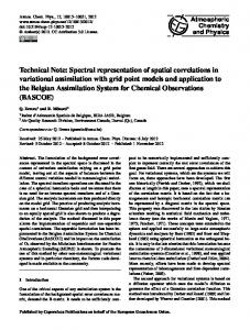
1/U Figure 2.2: Variational energies in the Hubbard model on a 98-site square lattice (in unit of J = 4t2 /U ), with only nearest neighbour coupling, at increasing U , for different variational wave functions. Empty triangles and empty rhombi correspond to energies computed using a simple mean-field |AFi wave function, with magnetic ordering along the z or the x direction, respectively. Full triangles correspond to energies computed adding a Jastrow factor parallel to the direction of the magnetic ordering z. Full rhombi correspond to energies computed using a Jastrow term orthogonal to the direction of the magnetic ordering x. The arrow indicates the variational energy obtained in the Heisenberg model using a spin-Jastrow factor (see Eq. (2.21) over the ground state of the magnetic Hamiltonian (2.20).

that now includes a kinetic term in addition to the magnetic one. The correlation factor acting on |AFi is the same spin-Jastrow term of Eq. (2.21), that ensures the correct spin-spin correlations at large distance. In Fig. (2.2), we show the variational energies, for increasing U, for the Hubbard model on a square lattice with only nearest neighbour hopping, using four different kinds of magnetic wave functions. Empty symbols correspond to energies computed using a simple mean-field |AFi wave function, with magnetic ordering along the x or the z direction. Only a small energy gain can be obtained by inserting a spinJastrow term (see Eq. 2.21), if the magnetic ordering, induced by the mean-field Hamiltonian, is in the z direction, parallel to the fluctuations induced by the Jastrow factor. On the contrary, if the magnetic ordering induced by the mean-field Hamiltonian is in the x direction, the accuracy in ground state energies is highly improved and, moreover, the variational energies in the Hubbard model extrapolate to the variational energy in the Heisenberg model, as U is increased. 27

At variance of the magnetically ordered phases, it is much more difficult to describe accurately a spin-liquid state in the Hubbard model, as we are going to present in the forthcoming sections. Since the variational state must contain charge fluctuations, the simplest generalization of the PG |BCSi wave function, introduced for the Heisenberg model, is to release the constraint of no-double occupancies, defining a soft Gutzwiller projector G [57]: X G = exp[−g ni,↑ ni,↓ ] . (2.25) i

This correlation factor takes into account that the expectation value of the energy in the Hubbard Hamiltonian contains a repulsive term for two electrons of opposite spins, located on the same lattice site. It is important to stress that this energy loss cannot be avoided within the simple |BCSi wave function; in fact it is not possible to suppress charge fluctuations, reducing the number of doubly occupied sites, within the BCS Hamiltonian and the Gutzwiller term is unavoidable. Numerical studies, done by using Quantum Monte Carlo [58, 59], and exact analytic treatments in one dimension [60] clarified that the Gutzwiller correlation factor is not sufficient to create an insulator in any finite dimension. In particular, for any finite U, the g parameter is finite, leading to a certain number of double occupancies, and the system turns out to be metallic. This is due to the fact that, once a pair of empty-doubly occupied sites is formed, these objects are free to move without paying any further energy cost, and, therefore, they can participate to the conduction events (In the forthcoming we will indicate empty sites as holons and doubly occupied sites as doublons). More specifically, at half-filling, holons are positively charged objects, while the doublons are negatively charged. When an electric field is applied to the system, they are free to move in opposite directions, and the system shows a metallic behaviour. In order to describe a metal-insulator transition at a finite value of U, early variational wave functions [61, 62], were constructed, introducing short-range correlations among empty and doubly occupied sites. However, these attempts failed to describe properly an insulating state and the description of a metal-insulator transition within a spin-liquid wave function was obtained only very recently by Capello et al. [20], inserting a long-range charge-Jastrow in the wave function: " # 1X J = exp v(rij )ni nj , (2.26) 2 i,j where v(rij ) = v(|ri −rj |) are variational parameters, which for isotropic 28

systems depend only on the relative distance among the particles, and ni is the particle density at position ri . The wave function describing a spin liquid in the Hubbard model reads |ΨSL i = J|BCSi, where |BCSi is the ground state of the Hamiltonian (2.22). It can be easily proved that the long-range coupling ni nj in the charge-Jastrow factor includes holon-holon and doublon-doublon repulsion as well as holon-doublon attraction, if v(rij ) < 0. Indeed, introducing the doublon Di = ni,↑ ni,↓ and the holon Hi = (1−ni,↑ )(1−ni,↓ ) operators, the Jastrow correlation ni nj can be written as: ni nj = Di Dj + Hi Hj − Hi Dj − Di Hj + ni + nj − 1 .

(2.27)

The Jastrow factor has a long story in physics, in particular the most interesting analytical and numerical results concerning the properties of the Jastrow wave function come from its wide applications in Helium physics. In this field it is worth mentioning the very early approach of McMillan [63], who used a parametrization of the Jastrow term coming from the solution of the corresponding two-body problem. The form of the Jastrow factor has been subsequently finetuned [64, 65, 66, 67] in order to reproduce accurately the properties of the 4 He liquid state. It turned out that, even if the ground-state energy is well approximated by using a short-range correlation term, the addition of a structure in the parameters v(rij ), at large distances, is fundamental to reproduce correctly the pair distribution function and the structure factor of the liquid. However, we observed that the wave function |ΨSL i = J|BCSi is poorly accurate in two dimensions, for strongly correlated lattice models, especially in presence of frustration. For example, in Fig. (2.3) we show the variational energy for the Hubbard model on the square lattice, using |ΨSL i as the trial wave function. We consider both the unfrustrated case with only nearest-neighbour hopping t and the frustrated case with a further next-nearest-neighbour coupling t′ . Especially in presence of frustration, the variational energies loose accuracy for increasing interaction U and do not match the variational energy of the corresponding Heisenberg models, obtained with a PG |BCSi wave function. In order to improve the accuracy of the |ΨSL i wave function in the Hubbard model, we introduce new correlation effects, that go beyond the Jastrow factor. We take the clue from the backflow contribution, whose relevance has been emphasized for various interacting systems on the continuum. 29

2.3

Backflow wave function

We mentioned in the previous section that the wave function describing a spin liquid state, |ΨSL i, can be poorly accurate in a 2D frustrated system. This is particularly evident in the strong-coupling regime. In fact, if we want to satisfy the single-occupancy constraint, which characterizes the highly repulsive limit of the Hubbard model, we need to apply the full Gutzwiller projector on top of the |ΨSL i wave function. In this way, charges are frozen in the lattice sites and there is no way to generate virtual hopping processes, by means of the kinetic term. The absence of the virtual hopping processes fails to reproduce the super-exchange physics, that is crucial in the strong-coupling regime. In this respect, we look for an improvement of the wave function that mimics the effect of the virtual hopping, leading us to the superexchange mechanism. Good candidates for this are the so-called backflow correlations, that were introduced a long time ago by Feynman and Cohen [21] to obtain a quantitative description of the roton excitation in liquid Helium. The term backflow came out because it creates a return flow of current, opposite to the one computed with the original wave function. Conservation of the particle current and the variational principle lead then to the optimal backflow. The backflow term has been implemented within quantum Monte

t’=0 t’/t=0.7

E/(4t2/U)

-0.9

-1

-1.1

-1.2 0

0.02

0.04

0.06

0.08

1/U

Figure 2.3: Variational energies in the Hubbard model (in unit of J = 4t2 /U ) using |ΨSL i as a trial wave function, for a 98-site lattice. We consider both the unfrustrated and the frustrated case with t′ /t = 0.7. Arrows indicate the variational results obtained by applying the full Gutzwiller projection to the |BCSi state for the corresponding Heisenberg models.

30

Carlo calculations to study bulk liquid 3 He [22, 23] and then applied to weakly correlated electron systems: Backflow correlations turned out to be crucial in improving the description of the electron jellium model both in two and three dimensions, in particular for correlation energies and pair distribution functions. Furthermore, backflow correlations were found to be important in determining the Fermi-liquid parameters [24, 25]. More recently, backflow has been applied also to metallic hydrogen [26] and to small atoms and molecules [27], where significant improvements in the total energy have been obtained. In all these contexts, the backflow term corresponds to consider fictitious coordinates of the particles (Helium atoms or electrons) r bα , which depend on the positions of the other ones, X ηα,β [x](r β − r α ) , (2.28) r bα = rα + β

where r α are the actual particle positions and ηα,β [x] are variational parameters depending in principle on all the coordinates {r α }, namely, on the many-body configuration |xi. The variational wave functions introduced in the previous section (spin liquid and magnetic ones) are constructed by means of single particle orbitals, defined as the eigenstates of an appropriate meanfield Hamiltonian. Now, these orbitals should be calculated in the new positions, i.e., φ(rbα ). However, since we work on a lattice, electron coordinates cannot vary with continuity so that Eq.(2.28) is not strictly applicable in practice. To overcome this problem, we introduced an alternative definition of backflow correlations by considering a linear expansion of each single-particle orbital: X cα,β [x]φk (r β ) , (2.29) φk (rbα ) ∼ φbk (r α ) ≡ φk (r α ) + β

where cα,β [x] are suitable coefficients. The next question is how to determine the coefficients cα,β [x]. In the Hubbard model, we can consider the U ≫ t limit, where a recombination of neighbouring charge fluctuations (i.e., empty and doublyoccupied sites) is clearly favoured and can be obtained by the following ansatz for the backflow term: X φbk (ri,σ ) ≡ η0 φk (r i,σ ) + η1 tij Di Hj φk (r j,σ ) , (2.30) j

where we used the notation that φk (r i,σ ) = h0|ci,σ |φk i are the eigenstates of the mean-field Hamiltonian, Di = ni,↑ ni,↓ , and Hi = hi,↑ hi,↓ , 31

with hi,σ = (1 −ni,σ ), so that Di and Hi are non zero only if the site i is doubly occupied or empty, respectively; finally η0 and η1 are variational parameters (we can assume that η0 = 1 if Di Hj = 0). As a consequence, the determinant part of the wave function already includes correlation effects due to the presence of the many-body operator Di Hj . This allows us to modify the nodal surface2 of the electronic wave function, a very important and new ingredient of the backflow term, considering that the so important and celebrated Jastrow factor can modify just the amplitude of the wave function. In the following sections, we will see that the ability of changing the nodes is crucial also to improve the accuracy within Green’s function Monte Carlo [15, 16]. Now it is worth mentioning that the correlation among holons and doublons, introduced in Eq. (2.30), is quite similar to the one present in a kind of Jastrow introduced by Shiba [62]: " #! X Y X Y JShiba = exp v Hi (1 − Dj ) , Di (1 − Hj ) + i

jn.n.i

i

jn.n.i

(2.31) in which the amplitude of the electronic wave function is suppressed when a doubly occupied site has no neighbouring empty sites. However, since in a Jastrow factor correlation effects are not included in the determinant part of the wave function, it turns out to be much less accurate than backflow correlations, as detailed later on. Furthermore, the simultaneous presence of a Shiba Jastrow and of a backflow term in the wave functions does not bring any improvement in the variational energy. A further generalization of the new “orbitals” can be made by taking all the possible virtual hoppings of the electrons: X φbk (r i,σ ) = η0 φk (r i,σ ) + η1 tij Di Hj φk (rj,σ ) +η2

X

j

tij ni,σ hi,−σ nj,−σ hj,σ φk (r j,σ )

j

+η3

X

tij (Di nj,−σ hj,σ + ni,σ hi,−σ Hj ) φk (r j,σ ) , (2.32)

j

where η0 , η1 , η2 and η3 are variational parameters. In particular, the term multiplied by η2 takes into account hoppings that create a new holon-doublon pair, while the term multiplied by η3 describes hoppings that do not change the total number of doubly occupied and empty 2

The nodal surface is the region where the electronic wave function changes its sign.

32

sites. While Eq. (2.30) preserves the spin SU(2) symmetry, the generalized equation (2.32) may break it. However, the optimized wave function always has a very small value of the total spin square, i.e. hS 2 i ∼ 0.001 for 50 sites. Moreover, we have noticed that, for example, in the region relevant for a spin liquid on a square lattice, Eq. (2.30) is already able to stabilize a disordered phase, while the additional parameters η2 and η3 give only a small improvement in the ground-state energy. As discussed in the next chapter, backflow correlations are less crucial in the magnetically ordered phases, with respect to the phase described by the BCS wave function, where backflow has been introduced to mimic the effect of the virtual hopping. In fact, a large value for the parameter ∆AF in the antiferromagnetic mean-field Hamiltonian is already able by itself to satisfy the single-occupancy (strong-coupling) constraint, forcing the electrons to lay in a magnetically ordered pattern. Then, the kinetic term in the mean-field Hamiltonian generates the virtual hopping processes, leading to the super-exchange mechanism.

2.4

Comparison with the S-matrix strong-coupling expansion

In the following, we present briefly how backflow correlations compare with a more traditional approach to deal with the strong-coupling regime, based on a unitary transformation [28] which eliminates the terms in the Hubbard model coupling sectors with different number of doubly occupied sites: [iS, H] [iS, [iS, H]] + + ... , (2.33) 1! 2! where H is the Hamiltonian of the Hubbard model and H′ is the transformed Hamiltonian. In particular, by truncating the expansion (2.33) at first order, the transformed Hamiltonian H′ can be mapped into the Heisenberg one. However, since we are interested in computing expectation values of operators, we can alternatively say that H′ = eiS He−iS = H +

hΨH′ |H′ |ΨH′ i hΨH′ |eiS He−iS |ΨH′ i hΨH |H|ΨHi = = , hΨH′ |ΨH′ i hΨH′ |ΨH′ i hΨH |ΨH i

(2.34)

where |ΨH′ i is the ground state of H′ and we define the ground state of the Hubbard Hamiltonian |ΨH i as: |ΨHi = exp(−iS)|ΨH′ i . 33

(2.35)

Wave function J|BCSi J|BCS+Backflowi (1 − iS)|RVBi Exact (Lanczos)

Energy -0.1317(1) -0.1519(1) -0.1432(1) -0.1577

Table 2.1: Variational energies for the Hubbard model on a 18-site square lattice at U/t = 30 and t′ = 0, using three different kinds of variational wave functions. Exact energy is given for comparison.

If H′ coincides with the Heisenberg Hamiltonian, |ΨH′ i is a fullyprojected state (with no doubly-occupied sites), that describes accurately a certain phase in the Heisenberg model. For instance, |ΨH′ i = |RVBi in the spin liquid phase stabilized for J2 /J1 ∼ 0.5. Though it is possible to define a recursive scheme for determining |ΨH i to any order of t/U, this kind of approach is rather difficult to implement for large clusters, since, in contrast to the Jastrow term, S is non diagonal in the natural basis |xi where the electrons with spins quantized along z occupy the lattice sites. However, at high values of U/t, we can approximate, at linear order, ΨH ∼ (1 − iS)|RVBi , where: S=

i X tij ni,−σ c†i,σ cj,σ (1 − nj,−σ ) + h.c. . U i,j

(2.36) (2.37)

Eq. (2.36) is not size-consistent and in fact, as size is increased, the variational energy obtained using (1 − iS)|RVBi as a variational wave function, looses accuracy. Indeed, already on a small 18-site square lattice, the variational energy in the Hubbard model with parameters U/t = 30 and t′ = 0 is lower for a J|BCSi trial wave function, with backflow correlations, than for the (1 − iS)|RVBi wave function (see Table 2.1). By increasing the system size to a 98-site lattice, the ground state energies computed with the (1 − iS)|RVBi wave function become even worse then the ones obtained within the simple |ΨSL i = J|BCSi wave function, as shown in Table (2.2), up to U/t = 80.

2.5

The minimization algorithm

The variational wave functions, introduced in the previous sections, depend, in general, on a set of variational parameters α = {αk }, appearing in both the correlation factor and the Slater determinant. These 34

Wave function J|BCSi J|BCS+Backflowi (1 − iS)|RVBi

Energy (U/t = 50) -0.0839(1) -0.09005(4) -0.0774(2)

Energy (U/t = 60) -0.0712(2) -0.07515(2) -0.0676(2)

Energy (U/t = 80) -0.0542(2) -0.05654(2) -0.0535(2)

Table 2.2: Variational energies at increasing U/t in the Hubbard model on a 98-site square lattice with only nearest-neighbour coupling, for three different trial wave functions.

parameters have to be optimized in order to minimise the expectation value of the variational energy: P 2 hΨ(α)|H|Ψ(α)i x |hx|Ψ(α)i| Ex = P ≥ E0 , (2.38) E(α) = 2 hΨ(α)|Ψ(α)i x |hx|Ψ(α)i|

where E0 is the actual ground-state energy and Ex is the so-called local energy, defined as: hx|H|Ψ(α)i Ex = . (2.39) hx|Ψ(α)i

Eq. (2.38) shows that the expectation value of the energy corresponds to the mean value of the local energy Ex , calculated among all the possible configurations |xi, each weighted according to the square modulus of the normalized wave function. As shown in a previous section, this can be done stochastically, summing over a Markov chain in configuration space. In the following, we present the so-called stochastic reconfiguration algorithm (SR) [51], that allows us to vary the parameters {αk }, in order to minimise the variational energy. Let us consider a starting trial wave function |Ψ(α0 )i, where α0 = {αk0 } is the set of p initial parameters (assuming that k = 1, . . . , p). In linear approximation, the new wave function |Ψ(α′)i, obtained after a small change of the parameters δα = α′ − α0 , can be written as: # " p p 0 X X ∂|Ψ(α )i δαk |Ψ(α′)i ≃ |Ψ(α0 )i + δαk Ok |Ψ(α0 )i , = 1+ ∂α k k=1 k=1 (2.40) where the operators Ok are defined, for any configuration |xi, as the logarithmic derivative of the wave function, with respect to the parameters αk : ∂lnhx|Ψ(α)i Ok (x) = . (2.41) ∂αk 35

Computing the logarithmic derivative can be quite complicated and we shall treat this problem later in the section. Defining O0 = 1 and δα0 = 1, Eq. (2.40) can be written in a more compact way: ′

|Ψ(α )i =

p X

δαk Ok |Ψ(α0 )i .

(2.42)

k=0

However, as a result of the iterative minimization scheme we are going to present, δα0 6= 1, and in this case the variation of the parameters will be obviously scaled δαk . (2.43) δαk → δα0 Now, the key point is how to determine the new set of parameters ′ {αk } so that, applying repeatedly Eq. (2.40), |Ψ(α′)i approaches the ground state. We take the clue from projection methods, that filter out the exact ground-state wave function, by iteratively applying the Hamiltonian operator to the trial ground state. In particular, we can apply the power method to the starting wave function: |Ψ′(α0 )i = PSR (Λ − H)|Ψ(α0 )i ,

(2.44)

where Λ is a large positive constant, that ensures convergence to the ground state and PSR is a projection operator over the (p+1)-dimensional subspace spanned by the basis {Ok |Ψ(α0 )i}, on which |Ψ(α′ )i has been expanded. Given this condition, we can equate Eq. (2.40) and Eq. (2.44): p X δαk Ok |Ψ(α0 )i ≡ PSR (Λ − H)|Ψ(α0 )i . (2.45) k=0

This procedure ensures that |Ψ(α′ )i has energy lower than |Ψ(α0 )i. Then, projecting each side of Eq. (2.45) along the k ′ -th component of the basis {Ok |Ψ(α0)i} we get: p X

δαk hΨ(α0)|Ok′ Ok |Ψ(α0)i = hΨ(α0 )|Ok′ (Λ − H)|Ψ(α0 )i .

(2.46)

k=0

The parameters δαk can be calculated by solving this linear system of (p + 1) equations, that can be written in a more compact way fk′ =

p X

δαk Skk′ ,

(2.47)

k=0

where fk′ are the generalized forces: fk′ = hΨ(α0 )|Ok′ (Λ − H)|Ψ(α0)i 36

(2.48)

and Skk′ is a (p + 1) × (p + 1) positive definite matrix given by: Skk′ = hΨ(α0 )|Ok Ok′ |Ψ(α0 )i .

(2.49)

The system can be reduced to p equations since δαo is related to the normalization of the wave function. Indeed, considering Eq. (2.46) for k ′ = 0, the value of δα0 reduces to: 0

δα0 = Λ − E(α ) −

p X

δαk Sk0 .

(2.50)

k=1

Substituting (2.50) in (2.46), for k ′ 6= 0, we obtain the reduced system of equations: p X (2.51) δαk S¯kk′ , f¯k′ = k=1

where:

f¯k = hΨ(α0 )|Ok |Ψ(α0 )ihΨ(α0)|H|Ψ(α0)i−hΨ(α0 )|Ok H|Ψ(α0 )i (2.52) and S¯kk′ = Skk′ − Sk0 Sk′ 0 .

(2.53)

. Since Now f¯k are proportional to the true forces, indeed f¯k = − 21 ∂E(α) ∂αk ¯ at equilibrium fk = 0, implying δαk = 0, we get that there is no variation in the set of parameters when the stability condition ∂E(α) =0 ∂αk is reached. The stochastic reconfiguration algorithm is similar to a standard steepest descent (SD) calculation, where the expectation value of the energy E(α) is optimized by iteratively changing the parameters {αk }, according to the corresponding derivatives of the energy: αk → αk + ∆tfk ,

(2.54)

where fk = −

∂E hΨ(α)|Ok H + HOk |Ψ(α)i =− ∂αk hΨ(α)|Ψ(α)i hΨ(α)|Ok |Ψ(α)ihΨ(α)|H|Ψ(α)i . +2 hΨ(α)|Ψ(α)i2

(2.55)

∆t is a suitable small time step, which can be taken fixed or determined at each iteration by minimizing the energy expectation value. Indeed, 37

the variation of the total energy ∆E at each step is easily shown to be negative for small enough ∆t because, in this limit, ′

∆E = E(Ψ(α )) − E(Ψ(α)) = −

p X

fk δαk + O(δαk2 ) =

k=1

− ∆t

p X

(2.56) fk2

2

+ O(∆t ) .

k=1

Thus the method certainly converges to the minimum when all the forces vanish. Similar considerations hold also for the stochastic reconfiguration algorithm. In fact, inverting Eq. (2.51), we get X −1 ¯ (2.57) S¯k,k αk → αk + ∆t ′ fk ′ , k′

where we added a parameter ∆t that can be tuned to control the change of the parameters. The energy variation for a small change of the parameters is given by: X −1 ¯ ¯ ∆E = −∆t (2.58) S¯k,k ′ fk fk ′ . k,k ′

It is easily verified that the above term is always negative because the ¯ as well as S¯−1 is positive definite, being S¯ an overlap reduced matrix S, matrix with all positive eigenvalues. For the SR and SD methods, a basic ingredient is that, at each ′ iteration, the new parameters α are close to the previous α, according to a prescribed distance. The fundamental difference between the two different techniques is just related to the definition of this distance ∆α . Within the SR scheme, ∆SR α is chosen to be the square distance between the two normalized wave functions, corresponding to the two different sets of variational parameters α and α′ : ′ 2 ∆SR α = ||Ψ(α )i−|Ψ(α)i| = 2−2 p

hΨ(α)|Ψ(α′)i hΨ(α)|Ψ(α)ihΨ(α′)|Ψ(α′i

. (2.59)

Inserting Eq. (2.40) in the previous one, we can express ∆SR α as a ¯ yielding function of the matrix S, X ′ ′ ∆SR S¯k,k′ (αk − αk )(αk′ − αk′ ) . (2.60) α = k,k ′

Generically speaking, the minimization procedures we introduced are examples of a constrained optimization, because in order to find the 38

minimum of the energy in a stable way, we want to keep the variations of the wave function small. This is equivalent to find the minimum of the functional X ′ ′ ¯ SR . (2.61) ¯ fk (αk − αk ) + Λ∆ F = ∆E + Λ||Ψ(α )i − |Ψ(α)i|2 = − α k

Then, the stationary condition δF /δ(αk′ −αk ) = 0 lead to the stochastic ¯ The reconfiguration scheme described in Eq. (2.57), with ∆t = 1/(2Λ). steepest descent algorithm can be obtained as the stationary condition of a similar functional, in which there is a less efficient definition of distance. In fact, ∆SD α is simply given by: ∆SD α

=

p X

(αk′ − αk )2 ,

(2.62)

k=1

that is just the square distance among the two set of parameters. The advantage of SR, compared with SD, is now clear: sometimes a small change of the variational parameters correspond to a large change of the wave function, and the SR takes into account this effect through Eq. (2.57). Now, it is worth to point out that, in order to compute the change in the variational parameters {δαk } within the SR scheme, it is necessary to invert the matrix S¯k,k′ , according to Eq. (2.57). If the eigenvalues of S¯ become too small, this leads to a divergence in the matrix ele−1 ments of S¯k,k ′ , making the minimization procedure unstable. In order to overcome this problem we use a combination of the Stochastic Reconfiguration and the Steepest Descent algorithm. Indeed, we define the change of the variational parameters {δαk } as: f¯k′ =

p X

δαk (S¯kk′ + ǫI) ,

(2.63)

k=1

where I is the identity matrix. Eq. (2.63) imposes a cut-off on the eigenvalues of S¯k,k′ , keeping the minimization procedure stable. Eq. (2.51) is solved stochastically with the Monte Carlo algorithm. In practice we perform MSR Metropolis steps in order to calculate the expectation values in Eqs. (2.52) and (2.53) with small enough fluctuations. Then, the linear system (2.51) is solved in order to find the variations δαk and the new set of parameters is calculated, according to: αk′ = αk0 + ∆tδαk , (2.64) where ∆t is a number that can be tuned in order to control the change of the parameters. Generally, one starts with a large ∆t in order to 39

reach the minimum in few iterations and then ∆t is decreased to reduce the fluctuations of the converged parameters. The new wave function |Ψ(α′ )i is then considered as the starting state |Ψ(α0 )i and the method is reiterated until convergence is achieved. Indeed, the stochastic nature of the system (2.51) implies that the forces f¯k are always determined with some statistical noise ηk and, even if the variational minimum is reached, the parameters will fluctuate around their mean values. Therefore, once convergence is reached, one must average over a certain number of iterations in order to find the optimal parameters. 2.5.1

The logarithmic derivative of the backflow parameters

In the last part of this section we address briefly the problem of computing the logarithmic derivative of the wave function with respect to the variational parameters. If a parameter αp is in the Jastrow factor, the logarithmic derivative is very easy to compute. For example, let us consider the spin-Jastrow factor defined by: " # 1X Js = exp vij Siz Sjz , (2.65) 2 i,j where S z is the z-component of the spin operator. The logarithmic derivative Ovij (x), with respect to a generic parameter vij , is simply equal to hx|Siz Sjz |xi, where |xi is the electronic configuration on the lattice. Computing the logarithmic derivative of a parameter defined in the mean-field Hamiltonian (like ∆AF or ∆BCS ) is much more difficult and we refer to [19] for a detailed description of the procedure. In this thesis, instead, we want to mention how to compute the logarithmic derivative for the backflow parameters, introduced in a previous section. We remember that the generic wave function for a correlated electron system can be constructed as the product of a Jastrow factor and the Slater determinant of a matrix Φk,i,σ ≡ φbk (r i,σ ), where the matrix elements, defined in Eq. (2.32), are the components of the new electron orbitals φbk , that include backflow correlations, over the sites i occupied by the N electrons on the lattice. The index σ accounts for the spin of the electron(s) occupying the site i. Then the logarithmic derivative Oηp (x), with respect to a generic backflow parameter ηp , reads: ∂ ∂ ∂ 1 det[Φ] = ln det[Φ] = Tr ln(Φ) = det[Φ] ∂ηp ∂ηp ∂ηp   −1 ∂Φ , = Tr Φ ∂ηp 40

(2.66)

∂Φ can be easily computed by differentiating every element of where ∂η p the matrix Φ with respect to the parameter ηp . Moreover, the inverse of the matrix Φ, required to compute the logarithmic derivative, does not cost extra computation time because it is already calculated for the Metropolis algorithm.

2.6

Green’s Function Monte Carlo

The Green’s Function Monte Carlo approach [15, 16] is based on a stochastic implementation of the power method technique that allows, in principle, to extract the actual ground state |ΨGS i of a given Hamiltonian H, from any starting wave function |Ψ0 i, provided that hΨGS |Ψ0 i = 6 0: |ΨGS i = lim (Λ − H)n |Ψ0 i . (2.67) n→∞

On large sizes it is not possible to evaluate exactly this recursive equation, because, after few steps, the application of Λ−H generates transitions to a very large number of different states, implying a huge amount of memory occupation. Therefore, we define a stochastical approach, in the sense that the wave function hx|Ψn i = hx|(Λ − H)n |Ψ0 i ,

(2.68)

is evaluated in a stochastic way. To this purpose, we define the socalled walker, which corresponds, at each iteration n of the Markov chain, to an electronic configuration |xn i with an associated weight ωn (roughly speaking associated to the amplitude of the wave function at |xn i, see below). The goal of the Green’s function MC approach is to define a Markov process, yielding, after a large number n of iterations, a probability distribution Pn (xn , ωn )3 for the walker, which determines the ground state wave function |ΨGS i. To be specific, in the most simple formulation we would require: Z dω ωn Pn (xn , ωn ) = hxn |Ψn i , (2.69) i.e., the amplitude of the wave function |Ψn i at xn is obtained by integrating, over all the weights ωn , the probability Pn (xn , ωn ). In order to construct a Markov chain for solving the ground state of the Hamiltonian H, it is necessary to assume that all the matrix elements of the so-called Green’s function Gx′ ,x = hx′ |Λ − H|xi = Λδx′ ,x − Hx′ ,x , 3

In the forthcoming we will indicate the electronic configuration |xi just as x.

41

(2.70)

are positive definite, so that they may have a meaning of probability. For the diagonal element Gx′ ,x there is no problem: we can always satisfy this assumption by taking a sufficiently large shift Λ. However, the requirement of positiveness is indeed important, and non trivial, for the non-diagonal elements of G, and is fulfilled only by particularly simple Hamiltonians. If it is not fulfilled, i.e., if Gx′ ,x < 0 for some pairs (x′ , x), we say that we are in presence of the so-called sign problem, that will be discussed in the following. Once positiveness is assumed to hold, we can divide up the Green’s function into the product of two factors: a stochastic matrix px′ ,x (by definition, a matrix with all P ′ ,x = 1) positive elements and with the normalization condition p ′ x x P ′ times a scale factor bx . Indeed, if we define bx = x′ Gx ,x to be such a scale factor, then px′ ,x = Gx′ ,x /bx is trivially positive and column normalized, and is therefore the stochastic matrix we are looking for. Now we are able to define a Markov process that leads to the condition (2.69) after a large enough number of iterations. Indeed, given (xn , ωn ) we can generate xn+1 with probability pxn+1 ,xn and update the weight according to ωn+1 = ωn bxn . This Markov process can be very easily implemented for generic correlated Hamiltonians on a lattice, since the number of non-zero entries in the stochastic matrix pxn+1 ,xn , for given xn , is small, and typically growing only as the number of lattice sites L. Now, it is immediate to verify that the conditional probability K of the new walker (xn+1 , wn+1 ), given the old one at (xn , wn ), is simply: K(xn+1 , ωn+1 |xn , ωn ) = pxn+1 ,xn δ(ωn+1 − ωn bxn ) .

(2.71)

Thus, the Master equation corresponding to the probability density Pn (xn , ωn ) is given by XZ Pn+1 (xn+1 , ωn+1 ) = dωK(xn+1 , ωn+1|xn , ωn )Pn (xn , ωn ) . (2.72) x

Finally, given Eq. (2.72) it can be proved, by means of the induction principle, that the following relation holds4 : Z dω ωn Pn (x, ωn ) . (2.73) ΨGS (x) = lim hωn δx,xn i = lim n→∞

n→∞

Now, within this formalism, we can compute Pthe ground-state energy, by averaging the random variable e(x) = x′ Hx′ ,x = Λ − bx . In 4

We can take as a starting probability distribution P (x0 , ω0 ) = δω−1 δx−x0 .

42

fact: hωn e(xn )i = hωn i

P

R

P dωn ωn e(xn )Pn (xn , ωn ) e(xn )Ψn (xn ) n P R = xP dωn ωn Pn (xn , ωn ) xn Ψn (xn ) Pxn P ′ ′ x Hx′ xn Ψn (xn ) ′ hx |H|Ψn i n = xP = Px , xn Ψn (xn ) xn Ψn (xn ) (2.74) xn

which, in the limit n → ∞ tends to the ground state energy, according to Eq. (2.73). However, in Eq. (2.74), the calculation of the energy, with the above described Green’s function technique, will not satisfy the zero variance property, which holds instead for the variational Monte Carlo we introduced before. In fact, the random quantity e(x), defined above, does not depend on any variational guess |Ψg i and, therefore, its statistical fluctuations cannot be reduced by a better wave function |Ψg i, as it is possible in the VMC case. 2.6.1

Importance sampling

It is possible to recover this important property of the variational Monte Carlo, by a slight modification of the iteration technique. To this purpose, it is enough to consider the so-called importance sampling Green’s function: ¯ x′ ,x = Ψg (x′ )Gx′ ,x /Ψg (x) . G (2.75) ¯ x′ ,x ≥ 0 for every (x′ , x) we can decompose it in the folWhenever G lowing manner, to define a Markov chain similar to the one we already introduced: ¯ x′ ,x /bx px′ ,x = G P ′ X (2.76) x′ Ψg (x )Hx′ ,x ¯ ′ Gx ,x = Λ − bx = = Λ − eL (x) , Ψg (x) x′ where eL (x) is the local energy already defined in Eq. (2.5). Now, if the trial wave function |Ψg i used in the importance sampling procedure coincides with the correct ground-state wave function, i.e. Ψg (x) = ΨGS (x), then eL (x) = EGS is a constant, and statistical fluctuations vanish exactly. All the previous derivations can be repeated also in this case with importance sampling, the difference being only appropriate factors depending on |Ψg i. We thus obtain for instance: hωn δx,xn i = Ψg (x)Ψn (x) 43

(2.77)

EGS

P hωn x′ Ψg (x′ )Hx′ ,xn /Ψg (xn )i hωn eL (xn )i = lim = = lim n→∞ n→∞ hωn i hωn i hΨg |H(Λ − H)n |Ψ0 i . = lim n→∞ hΨg |(Λ − H)n |Ψ0 i (2.78)

The zero variance property is evident form the previous equation. IneL (xn )i = EGS , with no statistical deed, if |Ψg i = |ΨGS i, En = hωnhω ni fluctuations. Since the convergence of the above limit is exponentially fast in n (at least for any finite size lattice, where a finite gap to the first excitation exists), it is enough to stop the iteration to a reasonably small finite n = l. Then, instead of repeating the Markov chain several times up to n = l, to accumulate statistics, it is clearly more convenient to average over a long Markov chain with N ≫ l, where N is the total number of iterations, and considering the corresponding estimates in Eq. (2.78): EGS ≃

PN

l n>n0 Qn eL (xn ) PN l n>n0 Qn

,

(2.79)

where n0 is the number of iterations required for the statistical equilibration of the Markov process and the weighting factors Qln are given by: l Y l Qn = bxn−i . (2.80) i=1

So, at each discrete time n−l we can take an equilibrated configuration, and consider l iterations of the Markov process with initial condition ωn−l = 1, leading, after l iterations, to a final weight ωl = Qln , at time n. 2.6.2

Forward walking technique

Besides energy, Green’s function Monte Carlo can be also used effib i.e., operciently to compute expectation values of local operators O, ators which are diagonal on all the elements of the configuration basis |xi, b O|xi = Ox |xi , (2.81)

where Ox is the eigenvalue corresponding to the configuration x. Also b for local operators we can define local estimators OL(x) = hΨhΨg |gO|xi = |xi Ox , but, in contrast with what happens for energy, we cannot write the 44

following equality: b GS i hΨg |O|Ψ hωn Oxn i = , n→∞ hωn i hΨg |ΨGS i

OGS = lim

(2.82)

b In fact, because the ground state is not an eigenstate of the operator O. b GS i , called mixed average, is obviously the quantity hOiMA = hΨhΨg |gO|Ψ |ΨGS i b like happens equal to OGS only if the ground state is an eigenstate of O, for the energy. In order to compute the mean value of a generic local operator b O over the ground state, we introduce the so-called forward walking i hωn Ox technique, i.e., OGS = limn→∞ hωnn−m . Indeed we have that: i b − H)n−m |Ψ0 i b GS i hωn Oxn−m i hΨg |(Λ − H)m O(Λ hΨGS |O|Ψ = → . hωn i hΨg |(Λ − H)n |Ψ0 i hΨGS |ΨGS i (2.83) From a statistical point of view, Eq. (2.83) amounts first to sample a configuration x after n − m Green’s Function Monte Carlo steps, then to measure the quantity hx|O|xi and finally to let the walker propagate forward for further m steps. In order to evaluate the stochastic average, an approach similar to that done for the energy is possible. Indeed, since the convergence of the above limit is exponentially fast in n, it is enough to stop the iteration to a reasonably small finite n = l, and then to average over a long Markov chain with N ≫ l, where N is the total number of iterations. In particular, in this case we get: EGS ≃

PN

n>n0

where Qln

=

Qln O(xn−m )

PN

n>n0

l Y

Qln

,

bxn−i .

(2.84)

(2.85)

i=1

In the above equation, ωn−l = 1 is assumed, implying that m ≤ l. However, we need a very large m to filter out the ground state from the left-hand side state hΨg |. An alternative approximate way to evaluate the mean value of a b over the ground state is to use the so-called generic local operator O Ceperley approximation: b GS i ∼ 2hOiMA − hOiVMC , hΨGS |O|Ψ 45

(2.86)

gi where hOiVMC = hΨhΨg |O|Ψ is the simple variational estimate correg |Ψg i sponding to |Ψg i. This approach is justified provided the variational wavefunction |Ψg i is very close to |ΨGS i, so that it can be written as |Ψg i = |ΨGS i + ǫ|Ψ′ i, with |Ψg i and |Ψ′ i normalized and ǫ ≪ 1.

2.6.3

Many walker formulation

Apart the aforementioned Ceperley approximation, the previously described procedures are, in principle, free from any approximation and they give exact results within the statistical errors (if the condition ¯ x′ ,x ≥ 0 holds). Unfortunately, the weight Ql grows exponentially by G n increasing l, implying a divergent variance in the energy average. Indeed, Qln is a product of l different factors and it can assume very large or very small values. This problem has a simple solution by considering the Green’s Function Monte Carlo technique with many walkers and by introducing a reconfiguration scheme, which enables to drop out the irrelevant walkers with small weights. Calandra and Sorella [16] have introduced a reconfiguration scheme working at fixed number of walkers, in a way that allows us to control the bias due to the finite walker population. We consider M walkers and label the corresponding configurations and weights with a couple of vectors (x, ω), with each component (xi , ωi), i = 1, . . . , M corresponding to the i-th walker. It is then easy to generalize the Master equation Eq. (2.72) to many independent walkers. If the evolution of P is done without further restrictions, each walker is uncorrelated from any other one, and we have: Pn (x1 . . . xM , ω1 . . . ωM ) = Pn (x1 , ω1 ) . . . Pn (xM , ωM ) .

(2.87)

Similarly to the previous case (2.73), we can define the state evolved ¯ at iteration n with the Green’s function G: P Z M X j ωj δx,xj 1 X Ψn (x)Ψg (x) = h ωi δx,xi i = [dω] Pn (ω, x) . M i=1 M x (2.88) where the symbol [dω] indicates the M dimensional integral over the ωi variables. Since we are interested in the state |Ψn i, we can define a reconfiguration process (that is the process of removing the most irrelevant walkers) that changes the probability distribution Pn without changing PM the statistical average h M1 i=1 ωi δx,xi i, that is relevant in the calculation of |Ψn i. This can be obtained by a particular Markov process applied to the configuration (x, ω), which leads to new walkers (x′ , ω ′ ). 46

Each new walker (x′j , ωj′ ), with j = 1, . . . , M, will have the same weight P ωj

j ωj′ = ω ¯= M and an arbitrary configuration x′j , among the M possible old configurations xk , k = 1, . . . , M, chosen with a probability pk P proportional to the weight of that configuration, pk = ωk / j ωj . It is clear that, after this reconfiguration, the new set of M walkers have by definition the same weights ωj = ω ¯ , and most of the irrelevant walkers with small weights have dropped out. It is also easy to derive the Master equation corresponding to this reconfiguration Markov process: XZ ′ ′ ′ Pn (ω , x ) = [dω]K(x′ , ω ′ |x, ω)Pn (ω, x) , (2.89)

x

where the kernel K is given by !  P P  M Y ′ ,x ω δ i x ωi i i j ′ ′ ′ P K(x , ω |x, ω) = . δ ωj − i M i ωi j=1

(2.90)

Let us note that K is simple, in this case, because all the new walkers are independent from each other, and K factorizes for each walker. We omit from the thesis the proof that this reconfiguration scheme does not influence the relevant average we are interested in. Such a proof can be found in [16]. 2.6.4

Fixed Node approximation

¯ x′ ,x ≥ 0 for every In a fermionic system the condition of positiveness G ′ (x , x) is not fulfilled in general. This is due to the antisymmetric nature of the fermionic wave function. Indeed, starting from a given wave function |Ψ0 i, we need to change its nodes in order to converge to the actual ground state |ΨGS i, recovering the correct sign. In principle, this can be done redefining the key ingredients of the Markov chain: ¯ x′,x |/|bx | px′ ,x = |G X ¯ x′ ,x |sx′ ,x , |G bx =

(2.91)

x′

¯ x′ ,x between the configwhere sx′ ,x is the sign of the Green’s function G ′ urations x and x. As a consequence, the weighting factor, appearing in the evaluation of energy and local operators, is modified as well: Qln

=

l Y

bxn−j sxn−j+1 ,xn−j .

j=1

47

(2.92)

However, this procedure is not applicable in practice, because the average sign, P l Q (2.93) hsl i = P n nl , n |Qn |

vanishes exponentially with l. Indeed, walkers with positive and negative weights cancel almost exactly, giving rise to an exponentially small quantity to sample, with huge fluctuations. A possible way to overcome this problem is the so-called fixed node approximation [17] that allows us to avoid the sign problem. In this approach, an effective Hamiltonian is defined, starting form H, by adding a perturbation O: Heff = H + O .

(2.94)

The operator O is defined through its matrix elements and depends upon a given guiding function |Ψi, which we can take as the best available variational state |ΨVMC i:

Ox′,x

  −Hx′ ,x 0 =  P

if x′ 6= x and sx′ ,x < 0 if x′ 6= x and sx′ ,x ≥ 0

ΨVMC y y:sy,x t′ , where the lattice can be described as a set of squares, formed by the bonds with hopping t, that are frustrated by the bonds with hopping t′ ; when t′ → 0 we approach the unfrustrated square lattice. In this case, by increasing U/t, after the metal-insulator transition, the system is found to be in a magnetically ordered phase. The standard Neel order on the squares formed by the bonds t is recovered. We compare our results with other numerical studies performed by Refs. [87] and [88]. In the second section of this chapter, we deal with the case t′ > t, in which the lattice can be seen as a set of chains, along which the electrons hop with an amplitude t′ , connected by the bonds with hopping 1

Since this compound is strongly interacting, it has been described by the Heisenberg model, using the spin coupling J, instead of the hopping t.

72

− ∆1

∆1

∆2

∆2

∆1

− ∆1

Figure 4.2: Symmetry of the BCS pairings along the triangular lattice, when t > t′ .

t; when t → 0 we approach a set of 1D decoupled chains. We identify the metal-insulator transition and, mainly, we observe signatures that the insulator is in a spin-liquid regime with one-dimensional features. This behaviour is favored by backflow correlations. A one-dimensional character for the ground state has been recently proposed also for the Heisenberg model [89, 90]. Moreover, the nature of our best state is compatible with a projected Fermi sea, since no long-range magnetic order parameter or superconductive pairing may be stabilized. According to Refs. [91, 92], a spin liquid described by a projected Fermi gas has a stable spinon Fermi surface, with low-lying spin excitations2 , that may lead to the linear temperature-dependent behaviour in the heat capacity, observed in a recent experiment [84].

4.1

The anisotropic triangular lattice with t > t′

We present, in this section, the anisotropic triangular lattice with t > t′ , focusing on the case t′ /t = 0.7. We start considering only the spinliquid solution |ΨSL i = J|BCSi, including also backflow correlations. The symmetry of the BCS pairing ∆1 has been chosen to be d−wave with dx2 −y2 symmetry, on the bonds connected by the hoppings t, between nearest-neighbour sites, as shown in Fig. (4.2). An additional small s−wave parameter ∆2 can be stabilized along the bonds connected by the hoppings t′ . This choice connects smoothly with the limit t′ → 0 in which the dx2 −y2 pairing function of the unfrustrated square lattice is recovered. Moreover, the symmetry of the superconductive pairing in the Hubbard model was studied in a recent paper 2

Charge excitations are gapped because we are in the insulating regime.

73

0.14

t’/t=0.7 0.12

N(q)/|q|

0.1 0.08

U6 U7 U8 U9 U10 U16

0.06 0.04 0.02 0 0

π/2

π

3π/2

|q|

Figure 4.3: Variational results for N (q) divided by |q| for a 144-site lattice at t′ /t = 0.7, using |ΨSL i as a trial wave function. The metal-insulator transition takes place between U/t = 8 and U/t = 9, where N (q) changes from a linear to a quadratic behaviour for |q| → 0.

[93], by means of the Gutzwiller approximation, observing that the dx2 −y2 symmetry is stable from t′ = 0 to t′ /t ∼ 0.9. In addition to ∆BCS , we optimize, in the trial wave function, also the hopping parameter t′wf along the dashed-line bonds of Fig. (4.2). We identify a metal-insulator transition, by looking at the densitydensity correlation factor N(q) = hn−q nq i. In Fig. (4.3), N(q) changes from a linear behaviour for |q| → 0, typical of a conducting phase, to a quadratic behaviour in the insulating regime at U/t & 8. The BCS pairing has a jump at a critical U below the metal-insulator transition, suggesting that a superconductive region may exist, sandwiched betwen the metallic and the insulating ones (see Fig. (4.4)). These results are quite in agreement with the ones obtained in Ref. [87], even if the metal-insulator transition is slightly shifted. However, when we take into account also the magnetic trial wave function |ΨAF i = Js J|AFi, with backflow correlations, the results are quite different. The magnetic order parameter is chosen to be the Neel antiferromagnetic one on the squares formed by the bonds with hopping t (see Fig. (4.5)). Comparing the variational results obtained with the spin-liquid wave function with the ones obtained by means of |ΨAFi, we observe that the metal-insulator transition is shifted to lower values of U/t and that the insulator is magnetically ordered, for every value of U/t, above the metal-insulator transition. Indeed, as shown in Fig. (4.6), for U/t . 6.5 |ΨSL i has lower energy than |ΨAF i and shows a 74

1

∆1/twf

0.8 0.6 0.4 0.2 0 5

6

7

8

9

10

U/t Figure 4.4: BCS pairing at increasing U/t on a triangular lattice with t′ /t = 0.7 and 144 sites.

Figure 4.5: Magnetic order relevant on the anisotropic triangular lattice when t > t′ . Spins are Neel antiferromagnetically ordered on the squares formed by the solid-line bonds.

75

-0.4

0.16

U7 |ΨAF> U6.5 |ΨAF> U6 |ΨSL> U5 |ΨSL>

0.14

-0.45

0.12

N(q)/|q|

E/t

-0.5 -0.55 -0.6

0.1 0.08 0.06 0.04

-0.65

|ΨSL> t’/t=0.7 |ΨAF> t’/t=0.7

-0.7 5

6

7

8

9

10

0.02

t’/t=0.7

0 11

0

U/t

π/2

π

|q|

Figure 4.6: Left panel: Variational energy for increasing U/t in the triangular lattice with t′ /t = 0.7 and 144 lattice sites. Two variational wave functions are compared: |ΨSL i and |ΨAF i. Right panel: Variational results for N (q) divided by |q|. Blue rhombi denote data for the |ΨAF i wave function, while red triangles denote data for the |ΨSL i wave function. The metal-insulator transition takes place between U/t = 6 and U/t = 6.5.

conducting behaviour, according to N(q). Moreover, as shown in Fig. (4.4) ∆1 /twf . 0.05, for U/t . 6.5, suggesting that long-range pairing correlations, if any, are tiny. On the contrary, for U/t & 6.5, the system is in an insulating state with Neel antiferromagnetic order and a sizeable ∆AF /twf ∼ 1.2. In order to confirm the magnetic nature of the insulating state, we have performed a Fixed Node calculation, taking |ΨSL i as the guiding wave function, for four different lattice sizes. We have calculated 2π ), the static spin-spin correlations S(q) = hs−q sq i for the point (0, √ 3 that corresponds to Neel antiferromagnetic order along the bonds with hopping t. Results are shown in Fig. (4.7) and indicate that the FN 2π approach is able to increase spin-spin correlations at Q = (0, √ ), even 3 when we consider the nonmagnetic wave function as an initial guess for the FN projection scheme. Indeed, S(Q)/L tends, in the thermodynamic limit, to a value very close to the one obtained for the unfrustrated square lattice (see Fig. (3.12)). Moreover, it is important to stress that our Fixed Node calculations for S(q) do not show evidence for any incommensurate peak, that would correspond to the formation of spiral magnetic order in the lattice. Since our results are quite in contrast with the ones obtained by Liu and coworkers [87], we should compare our best variational energies in the magnetic insulating phase with their ones for the spin-liquid insulator [94]. They used a J|BCSi wave function, with in addition 76

3π/2

0.15

S(0,2π/√3)/L

0.14 0.13 0.12 0.11 0.1 0.09 U=10, t’/t=0.7

0.08 0

0.04

0.08

0.12

0.16

0.2

-1/2

L

2π ) divided by the number of lattice Figure 4.7: Fixed Node results for S(0, √ 3 sites L = 36, 100, 144 and 196. All the calculations have been done by using the projected BCS wave function at U/t = 10 and t′ /t = 0.7. The line is just a guide to the eye.

the Jastrow introduced by Shiba (see Eq. (2.31)) to correlate holons and doublons. Moreover, they allowed for an extension of the hopping range in the variational wave function, beyond nearest neighbours, that turned out to be crucial to stabilize the superconducting phase, appearing between the metallic and the insulating regions. In Table (4.1), we show that our energies, at U/t = 8 and 10, which are obtained with a magnetic wave function, are much more accurate then the ones obtained with the Shiba Jastrow factor. Notice that the latter state would predict a spin liquid and a superconductor for U/t = 10 and 8, respectively. Also in the metallic region (U/t = 6) our results are more accurate. On the contrary, our work is quite in agreement with a recent paper [88], where a variational Monte Carlo study is performed on the triangular lattice with t′ ≤ t. In this paper, a first-order metal-insulator transition towards a state with Neel antiferromagnetic order has been observed from t′ = 0 to t′ /t ∼ 0.9. The trial state combines d−wave superconductive pairing with Neel order, through the Pfaffian ansatz. Remarkably, the authors noticed that their previous calculations, which predicted a robust superconductor and a nonmagnetic insulator [95], are modified by the stabilization of a magnetic phase. Finally, we remark that a commensurate magnetic ordering is in agreement with experimental data on k − (ET)2 Cu[N(CN)2 ]Cl, see Ref. [9]. 77

U/t 6 8 10

E/t (our work) -0.67204(4) -0.52383(3) -0.43365(3)

E/t (JJShiba |BCSi) -0.628(1) -0.386(1) -0.285(1)

Table 4.1: Comparison between variational energies at increasing U/t. Left column: Our best variational energies in the magnetic insulating region (U/t = 8, 10) and in the metallic region (U/t = 6). Right column: Energies obtained by Liu and coworkers [94], for the same values of U/t, using a JJShiba |BCSi wave function.

∆2

∆2

∆1

∆1

∆2

∆2

Figure 4.8: Symmetry of the BCS pairings along the triangular lattice, when t′ > t.

4.2

The anisotropic triangular lattice with t′ > t

The most interesting results on the triangular lattice appear in the regime t′ > t, which may be relevant for the experiment described in Ref. [11] and can give some insight also on the experiments performed by Kanoda and coworkers. Indeed, the compound k − (ET)2 Cu2 (CN)3 should lie in between the two regimes of the isotropic lattice and the anisotropic one with t′ > t. Our study is based on a Variational Monte Carlo approach, where we compare a spin-liquid solution |ΨSL i and an antiferromagnetic one |ΨAF i, including also backflow correlations. According to a detailed variational study on the Heisenberg model [19] and to a study of the superconductive pairing in the Hubbard model, by means of the Gutzwiller approximation [93], we have chosen the nearest-neighbour BCS pairing to be an extended s−wave with a parameter ∆1 along the bond t′ and a parameter ∆2 along the bonds with hopping t (see Fig. (4.8)). The antiferromagnetic order parameter couples the spins in a 78

y x

Figure 4.9: Collinear order on the triangular lattice with t′ > t. Couplings along the chains are antiferromagnetic.

collinear way along the x direction, with antiferromagnetic order along the chains (see Fig. (4.9)). This kind of magnetic order has been also recently proposed as the ground state for the Heisenberg model, when J ′ ≫ J [96]. As already mentioned, the existence of incommensurate spin ordering in the lattice is very difficult to assess in finite clusters and it will not be considered here. However, the presence of spiral order can still be probed by Green’s Function Monte Carlo, with the appearance of incommensurate peaks in the static spin-spin correlations S(q). Together with the BCS pairing and the magnetic order parameter, we optimize in the trial wave function also the hopping parameter twf along the solid-line bonds of Fig (4.8). A comparison among the variational energies, associated to the two wave functions, |ΨSL i and |ΨAFi, can be seen in Fig. (4.10), for two values of the frustrating ratio t/t′ = 0.7 and t/t′ = 0.5. In the second case, we show also the density-density correlation factor N(q) = hn−q nq i. For U/t′ . 4.5 the system is in a metallic state, without superconducting behaviour. Indeed, the optimized parameters ∆1 and ∆2 in |ΨSL i tend to zero, suggesting that the presence of BCS pairing does not bring any improvement in the variational energy. On the other hand, for U/t′ & 4.5 the system is in an insulating regime, where the trial wave function |ΨAF i gives an energy more accurate than the one associated to the solution |ΨSL i. The presence of a finite ∆AF in the variational wave function does not lead to a clear evidence of 2D magnetic order. In fact, by a more careful analysis of the variational parameters ∆AF and twf , we notice 79

-0.3 -0.35

U6 |ΨAF> U5 |ΨAF> U4 |ΨSL> U3 |ΨSL>

0.2

-0.4

N(q)/|q|

E/t’

-0.45 -0.5 -0.55 |ΨSL> t/t’=0.5 |ΨAF> t/t’=0.5 |ΨSL> t/t’=0.7 |ΨAF> t/t’=0.7

-0.6 -0.65 -0.7 3

4

5

6

7

8

0.15 0.1 0.05

t/t’=0.5 0 9

0

U/t’

π/2

π

|q|

Figure 4.10: Left panel: Variational energy at increasing U/t′ for a triangular lattice with t/t′ = 0.7 and t/t′ = 0.5, on a 144-site lattice. Two variational wave functions are compared: |ΨSL i and |ΨAF i. Right panel: Variational results for N (q) divided by |q| for the t/t′ = 0.5 case. The metal-insulator transition takes place between U/t′ = 4 and U/t′ = 5.

that the presence of backflow correlations, that strongly improve the accuracy of variational wave functions, reduces of an order of magnitude the antiferromagnetic order parameter ∆AF , acting against the formation of magnetic order in the system, see Fig. (4.11). Moreover, the optimized twf in the wave function is also strongly renormalized in presence of backflow correlations, converging to zero as U is increased. These facts suggest a one-dimensionalization of the system and the one dimensional nature of the optimized wave function is clearly in contrast with the presence of bidimensional long-range order. In order to analyze in more detail the effect of a finite ∆AF , we have compared our variational energy, when the trial wave function contains a finite, optimized, magnetic order parameter ∆AF , with the energy obtained within the spin-liquid guess for the ground state. For U/t′ & 10, the two energies coincide, within the error bar, and, remarkably, they are the same of a projected Fermi gas wave function, where no magnetic order parameter or BCS pairing is present. This result suggests that the ground state has no long-range magnetic order. On the contrary, for 5 . U/t′ . 8, a trial wave function with a finite ∆AF is favoured. However, following the same procedure adopted for the square lattice, we have considered the Fixed Node results for the static spin-spin correlations S(q) = hs−q sq i, using the non-magnetic wave function as the guiding one. Data show the absence of a long-range magnetic order in the lattice, even if there is an enhancement of spin-spin correlations at qx = π, corresponding to some antiferromagnetic coupling along the 80

3π/2

3.5

Backflow No Backflow

3

2

t/t’wf

∆AF/t’wf

2.5

1.5

t/t’=0.5

1 0.5 0 4

5

6

7

8

9

10 11 12

0.5 0.45 0.4 0.35 0.3 0.25 0.2 0.15 0.1 0.05 0

t/t’=0.5

Backflow No Backflow 4

U/t’

5

6

7

8

9

10 11 12

U/t’

Figure 4.11: Left panel: Optimized antiferromagnetic order parameter ∆AF , with and without backflow correlations, on a 144-site lattice with t/t′ = 0.5. Right panel: Optimized hopping integral twf , with and without backflow correlations, on a 144-site lattice with t/t′ = 0.5.

chains. Furthermore, there is no evidence of incommensurate peaks in S(q), that would correspond to the presence of spiral magnetic order in the lattice. The presence of a small ∆AF could be just an artifact of the variational approach on a finite size; indeed, the presence of a magnetic order parameter allows more freedom in constructing the single-particle orbitals, which are the eigenstates of our mean-field Hamiltonian. In this respect, an extension of the BCS pairing to larger distances could be a promising tool to reduce the energy of the non-magnetic state, making it competitive with the energy obtained by means of a trial wave function with a finite ∆AF . Indeed, a sizeable ∆BCS that couples sites at a distance of three lattice spacings along the chains has been shown to improve the variational energy in the quasi-1D Heisenberg model [19]. The peculiar spin-liquid behaviour, described above, must be compared to the case in which the one-dimensional chains are coupled in a non-frustrated way, sketched in Fig. (4.12). In order to show that, within the same variational approach, it is possible to detect a strong antiferromagnetic coupling between chains with similar values of t/t′ , but with a different geometry, we have compared two trial wave functions. The first one has a magnetic parameter such to induce antiferromagnetic correlations in both directions. The second one, instead, corresponds to have antiferromagnetic and ferromagnetic order along the strongest and the weakest bond, respectively. While the latter parameter is set to zero by the optimization procedure, the first one 81

t=0.5 t’=1 Figure 4.12: Square lattice with no rotation symmetry. Hopping integrals are t′ = 1 and t = 0.5.

converges to a finite value, of order unity, with a substantial improvement in the variational energy. This result suggests that, even if t′ is just one half of t, the square lattice is truly bidimensional, developing long-range antiferromagnetic Neel order. In order to give more evidences to the absence of long-range magnetic order in the anisotropic triangular lattice with weakly coupled chains, we have studied in more details the static spin-spin correlations S(q) = hs−q sq i. Following the same procedure adopted for the square lattice, we compare variational and Fixed Node results, by considering a non-magnetic wave function as the guiding one. In Fig. (4.13), we compare the static spin-spin correlations for the variational and for the Fixed Node calculations, at U/t′ = 10 and t/t′ = 0.5 for a 144-site lattice. For more clarity, we also show in Fig. (4.15) the data along a line of the Brillouin zone of the triangular lattice (the solid red line of Fig. (4.14)) In the variational calculation, S(q) shows a clear onedimensional behaviour: Spin-spin correlations are enhanced at qx = π, corresponding to antiferromagnetic correlations along the chains and are completely flat in the direction orthogonal to the chains. In the Fixed Node calculation, there is actually the formation of a small peak at (π, 0)3 , signaling the presence of some short-range bidimensional correlations. Indeed, even if there is a strong one-dimensionality in our system, some inter-chain coupling must be present, as detected by Fixed Node calculations for S(q). However, as shown in Fig. (4.16), this small peak does not give rise to any sizeable long-range order, since 3

The peak at (π, 0) corresponds to a kind of coplanar order in which the spins in each chain are antiferromagnetically ordered in the x direction or in the y direction, alternatively.

82

Figure 4.13: Left panel: Variational results for the static spin-spin correlations S(q) at U/t′ = 10 and t′ /t = 0.5. Lattice sites are 144. Right panel: Fixed Node results for the static spin-spin correlations S(q), with the same value of the parameters. Data are shown in the independent part of the Brillouin zone for the triangular lattice.

W

M

Q

Γ

S

P

Figure 4.14: Sketch of the independent part of the Brillouin zone for the triangular lattice. Labelled points have coordinates: Γ = (0, 0), S = (π, 0), 2π 2π √ 2π √π √ P = ( 4π 3 , 0), Q = (π, 3 ), M = ( 3 , 3 ) and W = (0, 3 ).

83

S(q)

1.2

1.2

1

1

0.8

0.8

0.6

0.6

0.4

0.4

0.2

0.2

0

Γ

0 S

P q

Q

S

Γ

S

P q

Q

Figure 4.15: Left panel: Variational results for the static spin-spin correlations S(q) along the red solid line of Fig. (4.14). Parameters are set to U/t′ = 10, t′ /t = 0.5 and 144 lattice sites. Right panel: Fixed Node results for the static spin-spin correlations S(q), with the same value of the parameters, along the red solid line of Fig. (4.14).

S(π, 0)/L approaches zero, or almost a very small value of magnetization, as the lattice size L is increased. Moreover, we would like to stress that there is no formation of incommensurate peaks in the Fixed Node calculations for S(q), as shown in Fig. (4.13). In conclusion, we have presented evidence that, in the anisotropic triangular lattice with t′ > t, long-range magnetic order is destroyed or almost strongly suppressed. Moreover, short-range correlations may be strongly one-dimensional, since the optimized hopping parameter in the wave function twf is renormalized to zero and static spin-spin correlations S(q) are enhanced for qx = π. The particular nature of the best trial wave function, where no relevant long-range magnetic order or superconductive pairing can be stabilized, suggests that the ground state of this system could be a projected Fermi gas. Following Refs. [91, 92], this kind of wave function has a stable spinon Fermi surface, with low-lying spin excitations, that may lead to the linear behaviour observed in the heat capacity of k − (ET)2 Cu2 (CN)3 , when T → 0 [84]. Also one-dimensionalization may explain the behaviour observed in Ref. [84], since one-dimensional chains with antiferromagnetic couplings are known to exhibit a large linear temperature-dependent contribution to the heat capacity.

84

S

0.016

S(π,0)/L

0.012

0.008

0.004

0 0

0.04

0.08

0.12

0.16

-1/2

L

Figure 4.16: Fixed Node results for S(π, 0) divided by the number of lattice sites L = 64, 144 and 256, at U/t′ = 10 and t/t′ = 0.5. All the calculations have been done by using a non-magnetic wave function as the guiding one. The line is just a guide to the eye.

85

86

Conclusions and perspectives In this thesis, we have treated the problem of strong correlation in 2D itinerant electron systems on a lattice. The primary interest in this subject comes from the fact that a sufficiently strong electron-electron repulsion may lead to unconventional phases. For example, in this limit, an insulating behavior with no magnetic order can be obtained, in contrast to what the independent-electron picture would naively predict. These insulators are usually called spin liquids and they naturally emerge in presence of frustrating interactions. Their behavior cannot be captured by any weak-coupling approach and novel techniques that may handle with strongly-correlated electrons are needed. In this respect, even simplified models, like the Hubbard one, where electrons hop among lattice sites and correlation is introduced through an on-site repulsive term U, cannot be exactly solved; then we need very accurate numerical techniques to describe their ground-state properties. A particularly insightful method is based upon the definition of a given variational ansatz, that defines an approximate ground-state wave function. Unfortunately, within previous conventional approaches, the accuracy of wave functions describing a spin liquid can be rather poor, especially in presence of frustration. Although a sufficiently long-range Jastrow factor is able to stabilize a disordered insulator [20], a magnetic ground state is always favoured in the insulating region. In order to overcome this problem, we have improved the trial wave functions by means of the so-called backflow correlations, which we have applied, for the first time, in a strongly correlated lattice model. This represents the first main result of the thesis. Backflow correlations allow us to get a remarkably accurate groundstate energy in different regimes, both for conducting and insulating phases. We have compared our results with other techniques that have been proposed in the recent past. Backflow correlations turn out to be the most accurate approach among all the ones are usually considered to deal with the Hubbard model. In particular, the backflow wave function gives better energies than the ones obtained by the recently introduced Pfaffian state that combines magnetism with superconduct87

ing pairing [29]. Furthermore, only by including backflow correlations, we are able to reach the strong-coupling limit without loosing accuracy [30]. The second main result of this thesis is the variational study of the ground-state properties for the Hubbard model on the square lattice with nearest and next-nearest neighbour hoppings [30], denoted by t and t′ , respectively. We have determined with great accuracy the metal-insulator transition, occurring in this model, and have discussed the properties of both phases. In the metallic region, we have presented evidence that there is no relevant long-range superconductive pairing. In the insulating regime, our remarkable result is the stabilization of a spin-liquid phase at strong coupling U & 14 and large enough frustrating ratio t′ /t ∼ 0.7. This result has been possible only by means of backflow correlations. Moreover, we have determined the boundaries of two magnetically ordered regions, the Neel antiferromagnetic one with pitch vector Q = (π, π) and the collinear one with pitch vector Q = (π, 0) or Q = (0, π). In particular, the insulator immediately close to the metallic region is magnetically ordered, with a first-order transition between the two magnetic phases at t′ /t = 0.78. We have compared our results on the square lattice with the ones obtained in Ref. [79], in which a similar variational Monte Carlo approach was used. We have shown that our ground-state energies are much more accurate than the ones obtained in Ref. [79]. Finally, in order to assess our variational results, we have applied Green’s Function Monte Carlo, confirming the magnetic properties in the insulating region. The third main result of this thesis is the study of the anisotropic triangular lattice [31]. We have considered two main regimes of anisotropy: the first one is the large inter-chain coupling limit, in which the lattice can be described as a set of squares coupled by t, frustrated by a weak diagonal bond t′ . In this case, we have determined the metal-insulator transition and we have shown that the insulating phase is always accompanied by a magnetic order. Moreover, the magnetic ordering stays commensurate even close to the isotropic point t′ = t. This result is in agreement with recent numerical calculations [88] and also with experiments performed in Ref. [9]. In the other case, that corresponds to a set of weakly coupled chains (i.e. t ≪ t′ ), we have presented evidence that the insulator does not show any magnetic order and, therefore, it is a spin liquid. The nature of the ground state is compatible with a projected Fermi-sea (no magnetic order or superconductive pairing can be stabilized in the meanfield Hamiltonian that defines the variational wave function). More88

over, the system shows a strong one-dimensional behaviour, since the inter-chain hopping parameter of the mean-field Hamiltonian is renormalized to a very small value. Most importantly, the static spin-spin correlations present one-dimensional features. The spin-liquid nature of the ground state is in agreement with recent experiments on compounds with a triangular crystal structure [9, 11]; moreover, according to Refs. [91, 92], a projected Fermi sea has a stable spinon Fermi surface, with low-lying spin excitations, that may lead to the linear behaviour in the heat capacity of k − (ET)2 Cu2 (CN)3 , when T → 0 [84]. Also one-dimensionalization may explain the behaviour observed in Ref. [84], since one-dimensional chains with antiferromagnetic couplings are known to exhibit a large linear temperature-dependent contribution to the heat capacity. In summary, the new variational technique that has been introduced in this thesis opens a lot of perspectives for future works. Indeed, we have shown that its great accuracy and, in particular, its ability to recover the super-exchange mechanism in the spin liquid wave function make it a suitable candidate to study strongly correlated models on frustrated lattices, both in 2D and in 3D. In particular, backflow correlations can help us in giving a definite answer about the complete phase diagram of the anisotropic triangular lattice, from the limit t′ → 0 (that corresponds to a square lattice) to decoupled 1D chains (t → 0). In this thesis, we have already presented important results in the two anisotropic regimes; immediate future work will be to treat the isotropic case, introducing a complex order parameter in the wave function, to reproduce the correct symmetries that are expected in this limit.

89

90

Acknowledgments First of all, I would like to thank my supervisor Prof. Sandro Sorella for his support during my Ph.D. studies, which took origin from his pioneering idea of applying backflow correlations to a strongly interacting electron system on the lattice. His ability to understand the physics lying beyond the numerics has always been enlightening for me. Then, I am also indebted to Federico Becca, who followed me during every-day work providing me with many useful tips. His incitements motivated me during these years, shaking, sometimes, my quietness :) Moreover, his careful reading of my thesis was of great help in improving the quality of the writing. I acknowledge Prof. Alberto Parola for providing me with exact results on small clusters and for the irony with which he faces research. I would like to mention also Manuela Capello for her help on the numerics during the early stage of this work. Finally, I thank all the people who made my life in Trieste a unique experience: Giuliano, for all the time spent together, my loved flatmates Carlotta, Valeria and in particular Marietta, that shared with me also the Ph.D. experience in Sissa, my great friends Mattia and Alice, my colleagues Paola, Marco S., Riccardo, Viet and Tatjana, Serena, Fabio, Lucio, Paolo, Francesco B., Marco M., Laura, Daniel, Nicola . . .

91

92

Bibliography [1] C. Kittel, Introduction to Solid State Physics, (John Wiley & Sons, Inc., 1953). [2] N.W. Ashcroft and N.D. Mermin, Solid State Physics, (Thomson Brooks/Cole, 1976). [3] G. Grosso and G. Pastori Parravicini, Solid State Physics, (Academic Press, 2000). [4] D. Pines and P. Nozi`eres, The theory of quantum liquids, (Westview Press, Boulder, Colorado, 1989). [5] N.F. Mott, Proc. Phys. Soc. (London) 62, 416 (1949). [6] M. Imada, A. Fujimori and Y. Tokura, Rev. Mod. Phys. 70, 1039 (1998). [7] R.M. Martin, Electronic Structure, (Cambridge University Press, 2004). [8] A. Fujimori, I. Hase, H. Namatame, Y. Fujishima, Y. Tokura, H. Eisaki, S. Uchida, K. Takegahara and F.M.F. de Groot, Phys. Rev. Lett. 69, 1796 (1992). [9] Y. Shimizu, K. Miyagawa, K. Kanoda, M. Maesato, and G. Saito, Phys. Rev. Lett. 91, 107001 (2003). [10] Y. Kurosaki, Y. Shimizu, K. Miyagawa, K. Kanoda, and G. Saito, Phys. Rev. Lett. 95, 177001 (2005). [11] R. Coldea, D.A. Tennant, A.M. Tsvelik and Z. Tylczynski, Phys. Rev. Lett. 86, 1335 (2001). [12] J.S. Helton, K. Matan, M.P. Shores, E.A. Nytko, B.M. Bartlett, Y. Yoshida, Y. Takano, A. Suslov, Y. Qiu, J.-H. Chung, D.G. Nocera and Y.S. Lee, Phys. Rev. Lett. 98, 107204 (2007). 93

[13] O. Ofer, A. Karen, E.A. Nytko, M.P. Shores, B.M. Bartlett, D.G. Nocera, C. Baines and A. Amato, cond-mat/0610540 (2006). [14] P. Mendels, F. Bert, M.A. de Vries, A. Olariu, A. Harrison, F. Duc, J.C. Trombe, J.S. Lord, A. Amato and C. Baines, Phys. Rev. Lett. 98, 077204 (2007). [15] N. Trivedi and D.M. Ceperley, Phys. Rev. B 41, 4552 (1990). [16] M. Calandra and S. Sorella, Phys. Rev. B 57, 11446 (1998). [17] D.F.B. ten Haaf, H.J.M. van Bemmel, J.M.J. van Leeuwen, W. van Saarloos, and D.M. Ceperley, Phys. Rev. B 51, 13039 (1995). [18] L. Capriotti, F. Becca, A. Parola, and S. Sorella, Phys. Rev. Lett. 87, 097201 (2001). [19] S. Yunoki and S. Sorella, Phys. Rev. B 74, 014408 (2006). [20] M. Capello, F. Becca, M. Fabrizio, S. Sorella, and E. Tosatti, Phys. Rev. Lett. 94, 026406 (2005). [21] R.P. Feynman and M. Cohen, Phys. Rev. 102, 1189 (1956). [22] M.A. Lee, K.E. Schmidt, M.H. Kalos, and G.V. Chester, Phys. Rev. Lett. 46, 728 (1981). [23] K.E. Schmidt, M.A. Lee, M.H. Kalos, and G.V. Chester, Phys. Rev. Lett. 47, 807 (1981). [24] Y. Kwon, D.M. Ceperley, and R.M. Martin, Phys. Rev. B 48, 12037 (1993). [25] Y. Kwon, D.M. Ceperley, and R.M. Martin, Phys. Rev. B 58, 6800 (1998). [26] M. Holzmann, D.M. Ceperley, C. Pierleoni, and K. Esler, Phys. Rev. E 68, 046707 (2003). [27] N.D. Drummond, P. L´opez R´ıos, A. Ma, J.R. Trail, G.G. Spink, M.D. Towler and R.J. Needs, J. Chem. Phys. 124, 224104 (2006); P. L´opez R´ıos, A. Ma, N.D. Drummond, M.D. Towler and R.J. Needs, Phys. Rev. E 74, 066701 (2006). [28] A. H. MacDonald, S.M. Girvin and D. Yoshioka, Phys. Rev. B 37, 9753 (1988). [29] J.P. Bouchaud, A. Georges and C. Lhuillier, J. de Physique 49, 553 (1988). 94

[30] L.F. Tocchio, F. Becca, A. Parola and S. Sorella, Phys. Rev. B 78, 041101(R) (2008). [31] L.F. Tocchio, F. Becca and S. Sorella, in preparation. [32] J.G. Bednorz and K.A. M¨ uller, Z. Phys. B 64, 189 (1986). [33] M. Foex, C. R. Hebd. Sean. Acad. Sci. B 223, 1126 (1946); D.B. McWhan and J.P. Remeika, Phys. Rev. B 2, 3734 (1970). [34] D.B. McWhan, A. Menth, J.P. Remeika, W.F. Brinkman and T.M. Rice, Phys. Rev. B 7, 1920 (1973). [35] R.H. McKenzie, Comments Condens. Matter Phys. 18, 309 (1998) and references therein. [36] P. Lecheminant, B. Bernu, C. Lhuillier, L. Pierre and P. Sindzingre, Phys. Rev. B 56, 2521 (1997); R. Budnik and A. Auerbach, Phys. Rev. Lett. 93, 187205 (2004). [37] J.T. Chalker and J.F.G. Eastmond, Phys. Rev. B 46, 14201 (1992). [38] Ch. Waldtmann, H.-U. Everts, B. Bernu, C. Lhuillier, P. Sindzingre, P. Lecheminant and L. Pierre, Eur. Phys. J. B 2, 501 (1998). [39] C. Castelnovo, R. Moessner and S.L. Sondhi, Nature 451, 42 (2008). [40] P.W. Anderson, Science 235, 1196 (1987). [41] X.-G. Wen Phys. Rev. B 65, 165113 (2002). [42] J. Hubbard, Proc. Roy. Soc. London A 276, 238 (1963). [43] M.C. Gutzwiller, Phys. Rev. Lett. 10, 159 (1963). [44] J. Kanamori, Progr. Theor. Phys. 30, 275 (1963). [45] E.H. Lieb and F.Y. Wu, Phys. Rev. Lett. 20, 1445 (1968). [46] T.A. Maier, M. Jarrell, T.C. Schulthess, P.R.C. Kent and J.B. White, Phys. Rev. Lett. 95, 237001 (2005). [47] J.E. Hirsch, Phys. Rev. B 31, 4403 (1985). [48] I. Affleck, J. Phys. A: Math. Gen. 31, 4573 (1998). 95

[49] S. Sorella, G.E. Santoro and F. Becca, SISSA Lecture notes on numerical methods for strongly correlated electrons, http://www.sissa.it/cm/index.php?contents=phd/phd_time.htm [50] N. Metropolis, A. Rosenbluth, M. Rosembluth, A. Teller and E. Teller, J. Chem. Phys. 21, 1087 (1953). [51] S. Sorella, Phys. Rev. B 64, 024512 (2001). [52] C. Lanczos, J. Res. Nat. Bur. Stand. 45, 255 (1950). [53] E.S. Heeb and T.M. Rice, Europhys. Lett. 27, 673 (1994). [54] P. Chandra and B. Doucot, Phys. Rev. B 38, 9335(R) (1988). [55] E. Manousakis, Rev. Mod. Phys. 63, 1 (1991); Z. Liu and E. Manousakis, Phys. Rev. B 40, 11437(R) (1989); F. Franjic and S. Sorella, Prog. Theor. Phys. 97, 399 (1997). [56] B. Edegger, V.N. Muthukumar and C. Gros, Adv. Phys. 56, 927 (2007). [57] M.C. Gutzwiller, Phys. Rev. Lett. 10, 159 (1963). [58] T.A. Kaplan, P. Horsch and P. Fulde, Phys. Rev. Lett. 49, 889 (1982). [59] H. Yokoyama and S. Shiba, J. Phys. Soc. Jpn. 56, 1490 (1987). [60] W. Metzner and D. Vollhardt, Phys. Rev. Lett. 59, 121 (1987). [61] P. Fazekas and K. Penc, Int. J. Mod. Phys. B 1, 1021 (1988). [62] H. Yokoyama and H. Shiba, J.Phys.Soc. Jpn. 59, 3669 (1990). [63] W.L. McMillan, Phys. Rev. 138, A442 (1965). [64] L. Reatto and G.V. Chester, Phys. Rev. 155, 88 (1967). [65] G. Gaglione, G.L. Masserini and L. Reatto, Phys. Rev. B 22, 1237 (1980). [66] P.A. Whitlock, D.M. Ceperley, G.V. Chester and M.H. Kalos, Phys. Rev. B 19, 5598 (1979). [67] T. MacFarland, S.A. Vitiello, L. Reatto, G.V. Chester and M.H. Kalos, Phys. Rev. B 50, 13577 (1994). [68] F. Becca, Ph.D. thesis (SISSA, Trieste), http://www.sissa.it/cm/phd.php 96

[69] J. Carlson, S.-Y. Chang, V.R. Pandharipande and K.E. Schmidt, Phys. Rev. Lett. 91, 050401 (2003); M. Bajdich, L. Mitas, G. Drobny, L.K. Wagner and K.E. Schmidt, Phys. Rev. Lett. 96, 130201 (2006). [70] C. Weber, A. Lauchli, F. Mila and T. Giamarchi, Phys. Rev. B 73, 014519 (2006). [71] M. Lugas, L. Spanu, F. Becca and S. Sorella, Phys. Rev. B 74, 165122 (2006); L. Spanu, M. Lugas, F. Becca and S. Sorella, Phys. Rev. B 77, 024510 (2008). [72] D. Eichenberger and D. Baeriswyl, Phys. Rev. B 76, 180504(R) (2007). [73] H.Q. Lin and J.E. Hirsch, Phys. Rev. B 35, 3359 (1987). [74] J.E. Hirsch, Phys. Rev. B 31, 4403 (1985); S. Sorella, S. Baroni, R. Car and M. Parrinello, Europhys. Lett. 8, 663 (1989). [75] T. Kashima and M. Imada, J. Phys. Soc. Jpn. 70, 3052 (2001). [76] H. Morita, S. Watanabe, and M. Imada, J. Phys. Soc. Jpn. 71, 2109 (2002). [77] T. Mizusaki and M. Imada, Phys. Rev. B 74, 014421 (2006). [78] M. Imada and T. Kashima, J. Phys. Soc. Jpn. 69, 2723 (2000); T. Kashima and M. Imada, J. Phys. Soc. Jpn. 70, 2287 (2001); T. Mizusaki and M. Imada, Phys. Rev. B 69, 125110 (2004). [79] H. Yokoyama, M. Ogata, and Y. Tanaka, J. Phys. Soc. Jpn. 75, 114706 (2006). [80] A.H. Nevidomskyy, C. Scheiber, D. Senechal, and A.-M.S. Tremblay, Phys. Rev. B 77, 064427 (2008). [81] M. Potthoff, M. Aichhorn and C. Dahnken, Phys. Rev. Lett. 91, 206402 (2003). [82] M. Capello, Ph.D. thesis (SISSA, Trieste), http://www.sissa.it/cm/phd.php [83] F. Becca, L. Capriotti and S. Sorella, Phys. Rev. Lett. 87, 167005 (2001) [84] S. Yamashita, Y. Nakazawa, M. Oguni, Y. Oshima, H. Nojiri, Y. Shimizu, K. Miyagawa and K. Kanoda, Nature Physics 4, 459 (2008). 97

[85] P. Sahebsara and D. S´en´echal, Phys. Rev. Lett. 100, 136402 (2008). [86] H.R. Krishnamurthy, C. Jayaprakash, S. Sarker and W. Wenzel, Phys. Rev. Lett. 64, 950 (1990). [87] J. Liu, J. Schmalian and N. Trivedi, Phys. Rev. Lett. 94, 127003 (2005). [88] T. Watanabe, H. Yokoyama, Y. Tanaka and J. Inoue, condmat/07111702 (2007). [89] Y. Hayashi and M. Ogata, J. Phys. Soc. Jpn. 76, 053705 (2007). [90] D. Heidarian, private communication. [91] O.I. Motrunich, Phys. Rev. B 72, 045105 (2005). [92] S.-S. Lee and P.A. Lee, Phys. Rev. Lett. 95, 036403 (2005). [93] B.J. Powell and R.H. McKenzie, Phys. Rev. Lett. 98, 027005 (2007). [94] N. Trivedi, private communication. [95] T. Watanabe, H. Yokoyama, Y. Tanaka and J. Inoue, J. Phys. Soc. Jpn. 75, 074707 (2006). [96] O.A. Starykh and L. Balents, Phys. Rev. Lett. 98, 077205 (2007).

98