A Non-backtracking Matrix Decomposition Algorithm for ... - TerpConnect

A Non-backtracking Matrix Decomposition Algorithm for Routing on Clos Networks John D. Carpinelli Member, IEEE Department of Electrical and Computer Engineering New Jersey Institute of Technology Newark, New Jersey 07102 and A. Yavuz Oru¸c Member, IEEE Department of Electrical Engineering University of Maryland College Park, Maryland 20740 ABSTRACT A number of matrix decomposition schemes were reported for routing on Clos switching networks. These schemes occasionally fail to find the right decomposition, unless backtracking is used. This paper shows that a partition may occur during the decomposition process and that this is the underlying reason these algorithms fail for some decompositions. It then presents a parallel algorithm which can recognize when a partition exists and set up the Clos network without backtracking.

1

Introduction

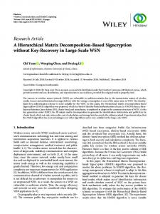
Three-stage Clos networks have been studied extensively in telephone switching theory [2, 6]. A number of backtracking set-up or routing schemes have been reported in the literature for these networks [3, 10, 11, 16]. As shown in Figure 1, a Clos network encompasses three stages where the first stage contains k switches, each of which has m inputs and n outputs. The second stage consists of n k × k cells, each of which receives exactly one input from each first-stage switch. By convention, the inputs to first-stage switch i (1 ≤ i ≤ k) are numbered from (i − 1) · m + 1 to i · m. Each cell can realize any mapping of its inputs onto its outputs, 1

1 m m+1 2m .. .

N -m+1 N

@ B @   B @ B @  B @ @ B @  B  B B  A

B A
A B A B
A B
 A
B 
A B 
A B 
A B 
AB 
AB 
AB A


.. .

@ B @   B @ B @  B @ @ B @  B  B B  A

B A
B A A B
A B
 A
B 
A B 
A B 
A B 
AB 
AB 
AB A


1 m m+1 2m .. .

N -m+1 N

Figure 1: 3-stage Clos network provided that no input is mapped onto more than one output and that no output has more than one input mapped onto it. The final stage has k n × m cells, each of which derives one input from each second-stage cell. A Clos network with these parameters is referred to as an (n, m, k) Clos network. It is known that if n ≥ m, the network is rearrangeable, and if n ≥ 2m − 1, the network is strictly non-blocking [6]. The number of inputs to the network is N = m · k. Routing is the process of setting the switches of a permutation network to realize a given permutation, or connection pattern from the inputs to the outputs. The looping algorithm is used frequently with Beneˇs networks [13, 18], but it does not generalize to all Clos networks. Andresen [1] developed an extension of the looping algorithm for Clos networks which have m = n = 2r , where r is a positive integer. However, a different approach is needed to route on all Clos networks. One promising approach is the matrix decomposition class of routing algorithms. Matrix decomposition algorithms make use of the design parameters of the Clos network.

2

Most algorithms in the matrix decomposition class start by deriving a k × k matrix Hm , where Hm [i, j] is the number of inputs to first-stage switch i which are to be routed to thirdstage switch j under the permutation to be realized. Because each first-stage switch has m inputs, the sum of the entries in each row is m; since each last-stage switch has m outputs, the sum of the entries in each column is also m. All of these algorithms are based on a principle which extracts a permutation matrix, Em , from Hm by forming the nonsingular matrix Hm−1 = Hm − Em , sets m = m − 1 and repeats the process until m=1, at which time H1 =E1 . The rationale behind this principle is the well-known Hall’s Theorem on systems of distinct representatives [8]. Consequently, by determining the setting for one second-stage switch, the problem of realizing a permutation on the original Clos network can be reduced to that of realizing a permutation on a Clos network with m − 1-input switches in its outer stages. The same procedure can be applied until the remainder network reduces to a single second-stage switch. By extracting a permutation matrix from Hm , matrix decomposition algorithms do just that. The extracted matrix, Em , defines the setting of one second-stage switch, and Hm−1 is the setting of the (n − 1, m − 1, k) Clos network. Em also induces a partial setting for each first(last)-stage cell. Most algorithms in the matrix decomposition class, with the exception of Neiman’s algorithm [12], do not successfully realize all possible permutations. These algorithms do not recognize the inherent partitioning that exist within the matrices for some permutations, and create an extraction matrix with one or more rows of all zero elements. This is due to a condition which occurs in the Hm matrix during the decomposition procedure. As a result of this, matrix decomposition algorithms generally require backtracking, which may include and remove an element from Em before the matrix is set. This is a bottleneck in matrix decomposition algorithms, and results in reduced routing speed. Ideally, a matrix decomposition algorithm should not use backtracking to route the Clos network. The remainder of the paper introduces the notion of partitioning which accounts for the failures of the matrix decomposition algorithms. It then gives a partitioning procedure which computes the Em matrix without any backtracking.

2

Partitioning

Partitioning can best be defined using an example. Given a Clos network with m = n = 4 and k = 5, the permutation 3

µ

p=

1 2 3 4 5 6 7 8 9 10 11 12 13 14 15 16 17 18 19 20 1 5 13 17 14 15 18 19 9 10 16 20 2 6 7 11 3 4 8 12

has the matrix



1 0  H4 =  0  1 2

1 0 0 2 1

0 0 2 1 1



1 2 1 0 0

1 2  1 .  0 0

A matrix decomposition algorithm would proceed by marking one non-zero entry, removing its row and column from the matrix, and repeating this on the remaining submatrix until it is null. The marked elements define the matrix to be extracted. For example, assume that H4 [1,1] is marked. Then the first row and first column are removed, and the submatrix left is     H4 =    

0 0 2 1

0 2 1 1

2 1 0 0

2  1 .  0 0

An algorithm might attempt to mark H4 [3,3], but this would result in the submatrix    H4 =    



0

2 2 

2 1

0 0 0

 .  0

Clearly, no permutation matrix can be derived from this matrix. The fault lies in the selection of H4 [3,3]. Once H4 [1,1] is chosen, columns 4 and 5 have non-zero entries only in rows 2 and 3. Therefore, any elements marked in columns 4 and 5 must be from rows 2 and 3. More importantly, however, any elements marked in rows 2 and 3 must be from columns 4 and 5. If H4 [3,3] is chosen, the only non-zero elements in columns 4 and 5 both appear in row 2. Since they cannot both be chosen, no permutation matrix can be derived which includes both H4 [1,1] and H4 [3,3]. Hence, H4 [3,3] is not a valid choice. These remarks are generalized in the following theorem. Theorem 1 Given an Hm matrix, let C be a set of some columns of the matrix, and let R be the set of all rows of Hm for which at least one column of C has a non-zero entry. If |C| = |R| then an element in a row of R may be marked if and only if it is in a column of C.

4

¶

Proof: Assume that |C| = |R|=x, i ∈ R, j 6∈ C and Hm [i, j] 6=0. To prove the theorem by contradiction, assume that Hm [i, j] is marked. Since no other element in row i may be marked, R ← R − i. Now |R| = x − 1. Since the columns of C have non-zero elements only in the rows of R, and only one element may be marked per row, at most x − 1 elements can be marked in the columns of C. Therefore, at least one column of C will not have any marked elements, and no permutation matrix can be formed. Hence, Hm [i, j] cannot be chosen, and the theorem is proved by contradiction.• The dual of this theorem is also true. Theorem 2 Given an Hm matrix, let R be a set of some rows of the matrix, and let C be the set of all columns of Hm for which at least one row of R has a non-zero entry. If |R| = |C| then an element in a column of C may be marked if and only if it is in a row of R. The proof is similar to that of the previous theorem. Note that any matrix which meets the conditions of Theorem 1 also meets the conditions of Theorem 2. These two theorems can be combined into one theorem, which is based on a fact given by Shapiro [17]. Theorem 3·Given ¸a matrix Hm , let P1 and P2 be k × k permutation matrices such that A B P1 Hm P2 = , where A is z × z, B is z × (k − z), C is (k − z) × z and D is C D (k − z) × (k − z). If there exist P1 and P2 such that B and/or C contain only zeroes, then an element in Hm may be marked if and only if it is in either A or D in P1 Hm P2 . Proof: Since P1 and P2 are permutation matrices, P1 Hm P2 is just a series of row and column exchanges of Hm ; entries are moved but not altered. If B contains all zeroes, then P1 Hm P2 contains z rows which have non-zero elements only in exactly z columns. Hm must also contain z rows which have non-zero elements only in exactly z columns, and the conditions of Theorem 2 are met. If C contains all zeroes, then P1 Hm P2 contains z columns which have non-zero elements only in exactly z rows, and the conditions of Theorem 1 are met. Note that if P1 and P2 can be chosen so that either B or C contains only zeroes, then there exist P10 and P20 such that P10 Hm P20 contain only zeroes in the other quadrant of the matrix.• These three equivalent theorems divide matrices into two classes: those which contain partitions and those which do not contain partitions. In the above example, after H4 [1,1] is marked, rows 4 and 5 have non-zero entries only in columns 2 and 3. By Theorem 2, an element in column 2 or 3 may be marked if and only if 5

it is in row 4 or 5. Thus, H4 [3,3] is not a valid choice. In effect, two submatrices are formed: one consisting of the rows and columns which meet the criteria of one of the theorems, and one consisting of the remaining rows and columns. For the above example, after H4 [1,1] is marked, the remaining matrix must be partitioned into 





     

 2 2    1 1  and    



 

2 1 1 1

   .  

Elements in these submatrices would be marked in the usual manner.

3

Why Jajszczyk’s algorithm fails

Jajszczyk’s algorithm [10] begins by setting up the matrix Hm in the usual manner. The number of zeroes in each row and column is counted, and an arbitrarily chosen non-zero element in the row or column with the most zeroes is marked. The row and column of the marked element are crossed out, the number of zeroes is recounted, and the process is repeated until all rows and columns are crossed out. The matrix to be extracted is the permutation matrix with ones at the marked positions. Consider the permutation below: µ

p=

¶

1 2 3 4 5 6 7 8 9 10 11 12 . 2 7 8 1 5 11 6 3 9 12 4 10

The matrix for this permutation is 

1 1 H3 =   1 0

0 1 1 1



2 0 1 0

0 1  . 0 2

Since two is the smallest number of non-zero elements in a row or column, any non-zero element in any row or column having this number of non-zero elements may be chosen. Arbitrarily, H3 [1,3] is chosen and marked. Row 3 and column 1 are deleted from the matrix leaving



∗

1   1

1 1 0 1 6



1  . 0 2

Column 4 has only two non-zero elements, so H3 [4,4] is selected. The algorithm continues, marking H3 [2,1] arbitrarily, and finally H3 [3,2]. The matrix, with the marked elements denoted by asterisks, is





1 0 2∗ 0  1∗ 1 0 1   H3 =   .  1 1∗ 1 0  0 1 0 2∗ Cardot [3] provided the following counterexample to Jajszczyk’s algorithm. Given the matrix 

0 0   0  1  0 H4 =   2  0   0  1 0

0 0 0 0 0 0 0 2 0 2

1 0 0 0 0 2 1 0 0 0

0 0 0 0 2 0 1 1 0 0

1 1 0 1 0 0 0 0 0 1

0 0 3 1 0 0 0 0 0 0

0 1 0 0 0 0 0 0 2 1

0 2 0 0 2 0 0 0 0 0

0 0 1 0 0 0 2 1 0 0



2 0  0   1  0   0  0   0  1 0

the algorithm could mark the elements H4 [3,6], H4 [5,8], H4 [6,1] and H4 [8,2], in that order. After removing the rows and columns of the marked elements, the matrix becomes          H4 =   ∗       

1 0 1 0 0 1



0 1

0 2 0 0 

0

0

∗ 0 0 1

∗

   1    .   0     1

1 1 0

0

2

0 0 0 0 0 1

2 1

0 0 0

∗

Obviously, choosing H4 [7,4] or H4 [7,9] is necessary, but either choice leaves a matrix with a column of zeroes. This prevents a permutation matrix from being found. Cardot’s counterexample shows the flaw in Jajszczyk’s algorithm after the second choice.

7

After two passes the matrix becomes 



0 0 1 0 1 0 0 0 0 1 

0 1

0 2 0 0 

0 0 0 1

0

0

0 0 0 2 1

0 2 1 0 0 0

   1   H4 =   2  0   0  1

0 0 2 0 0 2

2 1 0 0 0

0 1 1 0 0

0 0 0 0 1

   1    . 0  0   0  1

At this point, rows 1, 2, 4, 6 and 9 have non-zero entries only in columns 1, 3, 5, 7 and 10 of the remainder of the matrix. Applying Theorem 2, let R={1,2,4,6,9} and C={1,3,5,7,10}. Any element chosen from the columns of C must also be in the rows of R. Specifically, the matrix must be partitioned into two submatrices: one consisting of the rows and columns of R and C,and the other consisting of the other rows and columns. This yields the submatrices 

0 0     1     2       1

1 0

1 1

0 1

0

1

0

2

0

0

0

0





2 0 

         1        and    0             1

2



0 2

1 1

2 1

2

0

0

         .        

The second submatrix must be further partitioned to 



                 

                   and                 

1 1

2 1



          .        

2 Obviously Hm [10,2] is a required choice, and Hm [8,2] is an illegal choice. Once Hm [8,2] is marked by Jajszczyk’s algorithm, a permutation matrix can no longer be extracted. Note 8

that Jajszczyk’s algorithm could have chosen Hm [10, 2] instead of Hm [8, 2] and successfully found a permutation matrix without backtracking. The existence of a partition implies that an invalid choice can be made, but does not guarantee that it will be made. This partitioning is not necessarily unique, but any valid partitioning will ultimately determine that Hm [8, 2] is an invalid choice. This can easily be shown by contradiction. If Hm [8, 2] is marked, the matrix becomes 

0 0 

   1   H4 =   2  0     1

0

1 0 1 0 0 1



0 1

0 2 0 0 

0

0

∗ 0 0 1

∗

   1    . 0  0     1

2 0 0 1 1 0

0 0

0 2

0 0 0 0 0 1

2 1

0 0 0

∗

In this matrix, rows 1, 2, 4, 6, 9 and 10 have non-zero entries only in columns 1, 3, 5, 7 and 10. Since only one entry may be chosen in each row and column, at most five elements may be marked in these six rows. Therefore, one row will not have any marked elements and a permutation matrix cannot be formed. Hence, Hm [8, 2] is again an illegal choice. Despite this shortcoming, Jajszczyk’s algorithm provides an excellent strategy for making the arbitrary choices required by any matrix decomposition algorithm. It can make the matrix as sparse as possible, which leads to more partitioning later in the decomposition, and thus a faster routing. Jajszczyk’s algorithm will work for all permutations if a mechanism to recognize and act upon partitions is included.

4

Why Ramanujam’s algorithm fails

Ramanujam [16] uses a different matrix than the other algorithms in this class, but one that is related to the standard Hm matrix. The allocator matrix, M , has dimension k × k, and M [i, j] is the set of all destinations of inputs to first-stage switch j which are output at third-stage switch i. It is actually the transpose of Hm , with the entries listed rather than counted. The phase of the algorithm which extracts the desired matrix operates as follows. Set up a k × k matrix T , where T [i, j] is the maximum element of M [i, j], or 0 if M [i, j] is empty. 9

The largest element of T is marked, and its row and column are crossed off. This is repeated on the submatrix left in T until T is null or contains all zeroes. If T is null, the marked elements define a matrix for extraction; these elements are deleted from M , and the process is repeated until M is null. If T is not null, reform T , replacing the largest value with a zero, and repeat this stage, choosing the next largest element of T . Finally, a renumbering is performed to accommodate the author’s notation. For example, consider the Clos network with m = n = 3 and k = 4. The permutation to be realized is µ ¶ 1 2 3 4 5 6 7 8 9 10 11 12 p= , 2 7 8 1 5 11 6 3 9 12 4 10 the same permutation used previously. The allocator matrix M and the T matrix are 





{2} {1} {3} Φ 2 1  Φ  0 5 {5} {6} {4}   M =   and T =   {7, 8}  8 0 Φ {9} Φ Φ {11} Φ {10, 12} 0 11



3 0 6 4   . 9 0  0 12

Since 12 is the largest element of T , T [4,4] is marked, and row 4 and column 4 of T are deleted. The largest remaining element is 9, so T [3,3] is marked and its row and column are deleted. Continuing, T [2,2]=5 and T [1,1]=2 are chosen. Denoting each marked location with an asterisk, M becomes 



{2}∗ {1} {3} Φ  Φ {5}∗ {6} {4}   M =  .  {7, 8}  Φ {9}∗ Φ Φ {11} Φ {10, 12}∗ Kubale [11] gives the following counterexample to Ramanujam’s algorithm. Given a Clos network with m = n = 2 and k = 4, Ramanujam’s matrix for the permutation µ

p= is

The representation matrix is

1 2 3 4 5 6 7 8 3 5 1 4 2 6 7 8



¶



Φ {1} {2} Φ  {3} {4} Φ Φ   M =  .  {5} Φ {6} Φ  Φ Φ Φ {7, 8} 

0 3 T =  5 0

1 4 0 0 10

2 0 6 0



0 0  . 0 8

Since 8 is the largest element, T [4,4] is marked, and row 4 and column 4 are removed, leaving 

0 1 2 3 4 0 T =  5 0 6

   . 

T [3,3] would be chosen next, since 6 is the largest remaining element. T then becomes 



0 1 3 4 

  . 

T = 

Unfortunately, the algorithm then makes the only invalid choice, namely T [2,2]. Since the process fails, the algorithm sets the largest element of the original T matrix to 0 and tries again. For this matrix, T then becomes 

0 3 T =  5 0

1 4 0 0

2 0 6 0



0 0  . 0 0

No non-zero entry can be extracted from row 4 or column 4, and the algorithm cannot derive a matrix with exactly one non-zero entry in each row and column. Ramanujam’s matrix decomposition algorithm works for most, but not all permutations. It fails when it zeroes out an entire row or column; this is due to its inability to deal with partitions within the matrix. Had partitioning been used in Kubale’s counterexample, using any of the three theorems, the original representation matrix would have been partitioned into the submatrices



0 1 2 3 4 0   5 0 6







     and   

  . 

8 Ramanujam’s algorithm can handle this case once the matrix has been partitioned. Ramanujam’s algorithm can handle any permutation if a mechanism to recognize and act upon inherent partitions is incorporated into it. The added mechanism is actually sufficient in itself; Ramanujam’s algorithm would then serve as an heuristic to make arbitrary choices when no forced choice exists.

11

5

A partitioning algorithm

Any matrix which can cause backtracking in a matrix decomposition algorithm contains a partition. Any non-backtracking algorithm to perform a matrix extraction must be able to either determine when a partition exists and act accordingly or insure that no invalid choice is made if a partition exists. Neiman’s algorithm acts upon partitions by convolving the marked elements until the partitions are accounted for, though never recognized per se. An algorithm to recognize these partitions is given below. PROCEDURE PARTITION(Hm , Em ); 0 , partition exists, M , M ; var Hm 1 2

BEGIN 0 :=H ; E :=0; 1. Hm m m 0 6= Φ DO WHILE Hm BEGIN 2. partition exists:=FALSE; 0 , partition exists, M , M ); GENERATE PARTITION(Hm 1 2 IF (partition exists=FALSE) THEN 3a. BEGIN 0 [i, j] 6=0; Choose i, j such that Hm 0 0 Hm :=Hm \i, j; Em [i, j]:=1 END ELSE 3b. BEGIN PARTITION(M1 , E1 ); PARTITION(M2 , E2 ); 0 :=Φ Em :=Em +E1 +E2 ; Hm END END(while) END(procedure);

The algorithm works as follows. Step 1 initializes the variables. The WHILE loop, consisting of steps 2, 3a and 3b, adds elements to Em until it is a permutation matrix. Step 2 calls subroutine GENERATE PARTITION to check if a partition exists, i.e., if the conditions of Theorem 2 are met. If a partition exists, the subroutine forms the submatrices and returns them in M1 and M2 . If no partition exists, Step 3a marks an arbitrary non-zero element and 0 removes its row and column from Hm . If a partition does exist, Step 3b recursively processes 12

the two partition submatrices. The heart of the algorithm is subroutine GENERATE PARTITION. Here it is implemented as a highly parallel subroutine which checks all 2k possible sets of rows of the matrix. This subroutine is shown below. 0 , partition exists, M1 , M2 ); PROCEDURE GENERATE PARTITION(Hm

var R, C; BEGIN 1. M1 :=0; M2 :=0; 0 PARFOR each possible set of rows of Hm DO BEGIN 0 2. R:=the set of rows of Hm ; 0 C:=the set of all columns of Hm which have at least one non-zero element in a row of R; 3. IF |R| = |C| THEN BEGIN 0 M1 :=the rows and columns of Hm in R and C; 0 M2 :=the rows and columns of Hm not in R and C; partition exists:=TRUE END; END(parfor) END(procedure); This subroutine generates all possible sets R in parallel, and checks all possible partitions. Step 1 sets the parameters and begins the parallel executions. Step 2 checks the conditions of Theorem 2. If a partition exists, Step 3 forms the partition submatrices and sets partition exists. Once a partition is found, ALL parallel executions are immediately terminated. The subroutine exits and returns the values derived from the parallel execution which finds the partition. If more than one partition is found, the algorithm arbitrarily selects one and returns its values in M1 and M2 . To illustrate the execution of this algorithm, consider the matrix 

1 0 Hm =   2 0

0 2 0 1 13

2 0 1 0



0 1  . 0 2

0 Step 1 sets Hm =Hm and Em =0. Step 2 calls subroutine GENERATE PARTITION. Step 1 of the subroutine sets its parameters and begins the parallel executions. One of these executions has R = {1, 3}. Step 2 sets C = {1, 3}; since |R| = |C| = 2, Step 3 sets partition exists=TRUE, and

 

1

M1 =  

2

2 1





     and M2 =   



2

1 

1

2

. 

Returning to the main procedure, a partition does exist, so Step 3b recursively processes the two submatrices. This may result in 

1 0 E1 =   0 0 The final result is

0 0 0 0

0 0 1 0





0 0   0 0  and E2 =  0 0 0 0 

1 0  Em =  0 0

0 0 0 1

0 0 1 0

0 0 0 1

0 0 0 0



0 1  . 0 0



0 1  . 0 0

This algorithm will always generate the permutation matrix Em without backtracking. This is because a partition is recognized before an element is chosen, thus illegal choices are never made. The subroutine GENERATE PARTITION is exhaustive, so a partition is always found if one exists. The time complexity of PARTITION is dominated by the time complexity of subroutine GENERATE PARTITION, which is called k times in the worst case. If no partition exists, the subroutine checks all 2k possible sets of R the first time, 2k−1 sets the second time, and so on. For all k iterations, this can result in at most 2k+1 − 1 executions. Using one processor, the time complexity becomes T (k) = O(2k ). This time can be improved using more than one processor; however, there are constraints. One element of Em must be found before the next can be sought, so the k subroutine calls from PARTITION cannot overlap. The parallel branches in GENERATE PARTITION are totally independent, so the time complexity of the subroutine can be reduced to O(1) by using 2k processors. Thus, using 2k processors, the time complexity of PARTITION reduces to O(k). The performance of PARTITION depends on the value of k. In particular, this algorithm is most efficient when 14

k = O(lg N ), where N is the number of inputs to the Clos network. In this case, the time and hardware complexities of PARTITION are O(lg N ), and O(N ), respectively. Hence, when k = O(lg N ), one can decompose the Hm matrix without backtracking in logarithmic time and using a polynomial order of processors. As such this fact shows that the conjecture by Bassalygo and Neiman [10] does not hold for all values of k. We also note that the worst time and hardware complexities of PARTITION are O(N ) and O(2N ) which occur when k = O(N ).

6

Conclusions

Partitioning is an important characteristic of the matrix decomposition class of routing algorithms for Clos networks. This paper has demonstrated its applicability and used it to improve current routing algorithms. A separate algorithm has been developed which makes use of partitioning to find the extraction matrix Em . In spite of the high hardware cost, the partitioning algorithm compares well with other algorithms in its class. Neiman’s algorithm, the only other matrix decomposition algorithm which works for all permutations, has a runtime of O(k 2 m) for extracting one matrix [9]. The parallel version of the partitioning algorithm improves on this runtime, and does not require the backtracking used by Stage 2 of Neiman’s algorithm. The algorithms of Jajszczyk and Ramanujam are both faster than the partitioning algorithm, but do not work on all permutations. The partitioning algorithm can be used to make these algorithms realize all permutations, or they can be used to generate the arbitrary choices of i and j in the partitioning algorithm. Finally, we should note that, after we submitted this paper, we have found out from one of the referees that Gordon and Srikanthan [7] published an algorithm which they claimed to be nonbacktracking. However, Chiu and Siu [5] have reported an error in this algorithm. They also provided a modified version of the original algorithm which they claim to be correct based on simulation results, but without a proof. Unlike most matrix decomposition algorithms, the procedures in these papers use two matrices, rather than one, and are thus not directly amenable to the analysis presented in this paper.

Acknowledgements The authors thank the anonymous referees for their constructive remarks and suggestions. 15

References [1] S. Andresen, “The Looping Algorithm Extended to Base 2t Rearrangeable Switching Networks,” IEEE Transactions on Communications, vol. COM-25, no. 10. October, 1977. pp. 1057-1063. [2] V. E. Bene˘s, Mathematical Theory of Connecting Networks and Telephone Traffic, Academic Press Pub. Company, New York, 1965. [3] C. Cardot, “Comments on A Simple Control Algorithm for the Control of Rearrangeable Switching Networks,” IEEE Transactions on Communications, vol. COM-34, no. 4. April, 1986. p. 395. [4] J. Carpinelli, Interconnection Networks: Improved Routing Methods for Clos and Beneˇs Networks, Ph.D. thesis, Rensselaer Polytechnic Institute, Troy, NY, August, 1987. [5] Y. K. Chiu and W. C. Siu, “Comment: Novel Algorithm for Clos-Type Networks,” Electronic Letters, vol. 27, no. 6. March, 1991. pp. 524-526. [6] C. Clos, “A Study of Non-Blocking Switching Networks,” Bell Systems Technical Journal, vol. 32, no. 2. March, 1953. pp. 406-424. [7] J. Gordon and S. Srikanthan, “Novel Algorithm for Clos-Type Networks,” Electronic Letters, vol. 26, no. 21. October, 1990. pp. 1772-1774. [8] P. Hall, “On Representatives of Subsets,” Journal of the London Mathematical Society, vol. 10, 1935. pp. 26-30. [9] F. Hwang, “Control Algorithms for Rearrangeable Clos Networks,” IEEE Transactions on Communications, vol. COM-31, no. 8. August, 1983. pp. 952-954. [10] A. Jajszczyk, “A Simple Algorithm for the Control of Rearrangeable Switching Networks,” IEEE Transactions on Communications, vol. COM-33, no. 2. February, 1985. pp. 169-171. [11] M. Kubale, “Comments on Decomposition of Permutation Networks,” IEEE Transactions on Computers, vol. C-31, no. 3. March, 1982. p. 265 [12] V. I. Neiman, “Structure et command optimales de reseaux de connexion sans blocage,” Annales des Telecommunications, vol. 24. July-August, 1969. pp. 232-238. 16

[13] D. C. Opferman and N. T. Tsao-Wu. “On a Class of Rearrangeable Switching Networks, Part I: Control Algorithm,” Bell Systems Technical Journal, vol. 50, no. 5. May-June, 1971. pp. 1579-1600. [14] O. Ore, The Four-Color Problem, New York, Academic Press, 1967. [15] A. Y. Oru¸c, “Designing Cellular Permutation Networks through Coset Decompositions of Symmetric Groups,” Journal of Parallel and Distributed Computing, Academic Press Pub., Vol. 4, No. 2, Aug. 1987, pp. 404-422. [16] H. R. Ramanujam, “Decomposition of Permutation Networks,” IEEE Transactions on Computers, vol. C-22, no. 7. July, 1973. pp. 639-643. [17] L. W. Shapiro, Introduction to Abstract Algebra, New York, McGraw-Hill, 1975. [18] A. Waksman, “A Permutation Network,” Journal of the ACM, vol. 15, no. 1. January, 1968. pp. 159-163.

17