A NMS Method for Edge Detection with Sub-Pixel Accuracy. 1. Contents. 1 Introduction. 2. 2 On edge extraction. 3. 2.1 TheNMSmethod .
INSTITUT NATIONAL DE RECHERCHE EN INFORMATIQUE ET EN AUTOMATIQUE
A Non-Maxima Suppression Method for Edge Detection with Sub-Pixel Accuracy Fre´de´ric Devernay
N˚ 2724 Novembre 1995
PROGRAMME 4
ISSN 0249-6399
apport de recherche
A Non-Maxima Suppression Method for Edge Detection with Sub-Pixel Accuracy Fre´de´ric Devernay Programme 4 — Robotique, image et vision Projet Robotvis Rapport de recherche n˚2724 — Novembre 1995 — 20 pages
Abstract: In this article we present a two dimensional edge detector which gives the edge position in an image with a sub-pixel accuracy. The method presented here gives an excellent accuracy (the position bias mean is almost zero and the standard deviation is less than one tenth of a pixel) with a low computational cost, and its implementation is very simple since it is derivated from the well-known Non-Maxima Suppression method [2, 4]. We also justify the method by showing that it gives the exact result in a theoretical one dimensional example. We have tested the accuracy and robustness of the edge extractor on several synthetic and real images and both qualitative and quantitative results are reported in this paper. Key-words: Low-level processing, Edge detection, Sub-Pixel, Differential properties of curves.
(Re´sume´ : tsvp)
Unite´ de recherche INRIA Sophia-Antipolis 2004 route des Lucioles, BP 93, 06902 SOPHIA-ANTIPOLIS Cedex (France) Te´le´phone : (33) 93 65 77 77 – Te´le´copie : (33) 93 65 77 65
De´tection de contours a` une pre´cision infe´rieure au pixel par une me´thode de´rive´e de la NMS Re´sume´ : Nous pre´sentons un de´tecteur de contours bidimensionnels qui donne la position du contour dans une image a` une pre´cision infe´rieure au pixel. La me´thode pre´sente´e ici donne d’excellents re´sultats (la moyenne de l’erreur en position est presque ze´ro et son e´cart type est d’a` peine un dixie`me de pixel) pour un couˆt en calcul a` peine supe´rieur a` une me´thode classique, et de plus son implantation est tre`s simple puisqu’elle est de´rive´e de la me´thode classique de suppression des non-maxima locaux (NMS) [2, 4]. Nous justifions e´galement l’utilisation de cette me´thode en montrant qu’elle donne le re´sultat exact dans le cas d’un contour monodimensionnel. Nous avons teste´ la pre´cision et la robustesse de cet extracteur de contours sur plusieurs types d’images, synthe´tiques et re´elles, et rapportons ici des re´sultats a` la fois qualitatifs et quantitatifs. Mots-cle´ : de´tection de contours, sous-pixel, proprie´te´s diffe´rentielles de courbes.
A NMS Method for Edge Detection with Sub-Pixel Accuracy
1
Contents 1 Introduction
2
2 On edge extraction 2.1 The NMS method . . . . . . . . . . . . . . . . . . . . . . . . . . . 2.2 The sub-pixel approximation . . . . . . . . . . . . . . . . . . . . .
3 3 3
3 Using the proposed improvements
7
4 Results 4.1 The test data . . . . . . . . . . . . . . 4.2 The different edge detection methods . 4.3 Edge position . . . . . . . . . . . . . 4.4 Edge orientation . . . . . . . . . . . . 4.5 Other results . . . . . . . . . . . . . . 5 Conclusion
RR n˚2724
. . . . .
. . . . .
. . . . .
. . . . .
. . . . .
. . . . .
. . . . .
. . . . .
. . . . .
. . . . .
. . . . .
. . . . .
. . . . .
. . . . .
. . . . .
. . . . .
8 8 10 10 12 15 15
2
Fre´de´ric Devernay
1 Introduction Edge detection is now taken for granted by most of the computer vision people, like many other basic tools of computer vision. Since a lot of work has already been done in early vision, people working on higher level features tend to use as input the result of classic low level algorithms and think this is the only information they can get from the image data. In the case of edge detection we used to work on information that was given to within about a pixel, and then had to do some kind of regularization process on it, like polygonal or spline approximation. Both introduce a certain quantity of error, but whereas the approximation error can be chosen, the error on the detected edge position is both fixed and not negligible, especially when one wants to compute differential properties of image curves like orientation, Euclidean curvature or even higher degree properties like affine or projective curvature. Some attempts were made in edge detection at a sub-pixel accuracy a few years ago, for example A. Huertas and G. Medioni [11] used a refinement of the zero-crossing of Laplacian but they did not give any results on the accuracy of the edge detection. A.J. Tababai and O.R. Mitchell [14] did some interesting work in the one-dimensional case which was extended to two-dimensional images and seemed to work properly. An edge relocation mechanism is also given in [15] but the required implementation is rather complex. The best results in terms of accuracy [12] were obtained at a high computational cost, because this involved local surface fitting on the intensity data, and the results are not better than our method. In general, the different methods that have been proposed often end up requiring regularization, excessive computer power, or both of them. For these reasons we made a very simple enhancement of the classical local nonmaxima suppression, that gives a much better estimate of the curve position (up to within a tenth of a pixel) or the curve orientation without regularization, and at a very low computational cost. Using this edge detector, we can also calculate higher order differential properties of curves with much less regularization than when using older methods. Besides, this method can be easily integrated in an existing vision system since it is based on a classical and widely-used method. We present and interpret a wide variety of results to compare this method with existing edge detection methods. We also calculated in the most simple way the local edge orientation to show that the result of our method can also be used to easily calculate differential properties of the edges.
INRIA
A NMS Method for Edge Detection with Sub-Pixel Accuracy
3
2 On edge extraction 2.1
The NMS method
This method is based on one of the two methods commonly used for edge detection, the suppression of the local non-maxima of the magnitude of the gradient of image intensity in the direction of this gradient [8] (also called NMS), the other one being to consider edges as the zero-crossings of the Laplacian of image intensity [10, 9]. NMS consists of: 1. Let a point (x; y), where x and y are integers and I (x; y) the intensity of pixel (x; y ). 2. Calculate the gradient of image intensity and its magnitude in (x; y). 3. Estimate the magnitude of the gradient along the direction of the gradient in some neighborhood around (x; y). 4. If (x; y) is not a local maximum of the magnitude of the gradient along the direction of the gradient then it is not an edge point. Usually for step 4 the neighborhood is taken to be 3 � 3 and the values of the magnitude are linearly interpolated between the closest points in the neighborhood, e.g. in Figure 1 the value at C is interpolated between the values at A7 and A8 and the values at B between those at A3 and A4 . We have also tried to use quadratic interpolation to compute these (the value at A would be interpolated between those at A7, A8, and A1 as in Figure 2) and compared the results with the linear interpolation. After this edge detection process one usually does hysteresis thresholding [2] on the gradient norm and linking to get chains of pixels.
2.2
The sub-pixel approximation
Our main improvement of the method is very simple and consists of only adding this single step to the NMS process:
�
If (x; y) is a local maximum then estimate the position of the edge point in the direction of the gradient as the maximum of an interpolation on the values of gradient norm at (x; y) and the neighboring points.
RR n˚2724
4
Fre´de´ric Devernay
A1
A2
A3 g
B
A A8
A4
C A7
A6
A5
Figure 1: Checking whether pixel A is a local maximum of the magnitude of the gradient in the direction of the gradient is done by interpolating the gradient magnitude at B and C .
B A
−1
x
0
1
Figure 2: Examples of linear (A) and quadratic (B ) interpolation between three values at ?1, 0, and 1.
INRIA
A NMS Method for Edge Detection with Sub-Pixel Accuracy
5
This is the principle, but we still have to find the interpolation between gradient norm values we should apply to find the best position of the edge. We will consider a simple quadratic interpolation of the values of the gradient norm between the 3 values we have in the gradient direction. One could also try to locally fit a simple surface (e.g. bi-quadratic) on the neighborhood of the considered point but we want to keep the computations as simple as possible so that the implementation is fast and easy. The choice of the quadratic interpolation to find the maximum can be justified because it gives the exact result in the one-dimensional case. Let L = fl(i)ji 2 @g an infinite line of pixels with a step edge at position �? 12 , coordinate 0 corresponding to the middle of pixel l(0). The continuous intensity function for this step edge, as shown in Figure 3, is: ( t > � ? 12 I (t) = 01 ifotherwise so that
l(i) =
R 21
? 21 I (t)dt
l(?1) = � � � = l(?2) = l(?1) = 1 l(0) = �; 0 � � � 1 l(1) = l(2) = � � � = l(+1) = 0 I(t) t l(i)
i
Figure 3: A one-dimensional step edge and the corresponding gray-level pixel line. Let r be a general derivation operator. It can be a finite differences operator, or any gradient filtering operator, the only constraint being that r is antisymmetric. It can be written:
rl(i) =
+1 X k=1
RR n˚2724
gk (l(i+k)?l(i?k)) = � � �?g2l(i?2)?g1 l(i?1)+g1 l(i+1)+g2l(i+2)+� � �
6
Fre´de´ric Devernay
?1; 0; 1: � � � ? g2 ? g1 + g1 � = C ? (1 ? �) g1 � � � ? g 2 ? g1 = C ? g 1 � � � ? g 2 ? g1 � = C ? � g 1
Let us apply this general derivation operator on locations
rl(?1) = rl(0) = rl(1) = where
C=?
1 X k=2
gk
Since shifting and rescaling the values of the three points used to find a maximum of the quadratic interpolation do not affect the position of this maximum, we can simplify things by using C = 0 and g1 = 1:
a = jrl(?1)j b = jrl(0)j c = jrl(1)j
=1
?�
=1 =
�
Considering that the center of the pixels correspond to integer x coordinates, one can find that the x position of the maximum of the parabola passing through (?1; a), (0; b), and (1; c) is:
m = 2(a ?a ?2bc+ c) :
(1)
It can be easily seen that when b � a and b � c this value is bounded:
?0:5 � m � 0:5 Since integer coordinates correspond to pixel centers and pixel width is 1, this means that the sub-pixel position of an edge point will always be inside the pixel. That gives in this case
m = � ? 12
which is exactly the theoretical position of the edge! Equation 1 shows that the edge position is invariant to additive and multiplicative changes in the data. Moreover, this result can be extended to any kind of smooth edge, since a smooth edge is the result of the convolution of a step edge with a symmetric blurring operator s. The
INRIA
A NMS Method for Edge Detection with Sub-Pixel Accuracy
7
blurring operator s is symmetric so the action of the derivation on the ramp edge is the same as the action of the convolution of this operator with the blurring operator, which can be considered as another derivating operator, on the corresponding step edge:
r(s � l)(i) = (r � s)l(i) = r0l(i) We should be careful about one thing with the previous computations: we worked with the gradient norm, whereas most people might want to use the squared gradient norm for NMS because it requires less calculations and when the squared gradient norm is a local maximum the gradient norm is one too. But the quadratic interpolation gives a different result, and in the previous case we would find the maximum at:
m = 4�21??42��? 2
which introduces a bias on the edge position. The maximum of the bias is �m = 0:073 pixels at � = 0:19 and its standard deviation is � (�m) = 0:052, that is more 1 pixel (the same magnitude order as the precision we would like to get). In than 20 conclusion, using the squared gradient norm may reduce significantly the precision of the edge extraction. The comparison between the detected and the theoretical edge position was not done in the two dimensional case because it involves too many parameters (including the position and angle of the edge, the coefficients of a generic two-dimensional derivating filter, and the way the values a and c are calculated). Before seeing some results let us see how this edge detector can be used in a classic image processing chain.
3 Using the proposed improvements The main advantage of this new method over the sub-pixel edge detectors that have already been done is that its cost in terms of calculation is almost nothing (3 additions and 3 multiplications at each detected edge point if we use the quadratic approximation, which make 6 floating-point operations, not including the computation of the gradient) and it can be easily integrated in a simple and well-known algorithm.
RR n˚2724
8
Fre´de´ric Devernay
The new problem that can appear with a sub-pixel edge detector is that because the point coordinates are not integer we may not be able to apply common techniques such as hysteresis thresholding or linking. Hopefully we have solved this problem the simplest way we could: with this edge detector an edge point has non integer coordinates but can still be attached to the point from which it was calculated, which has integer coordinates. Thus we perform the common operations on the edge points as if they had integer coordinates, like hysteresis thresholding [2] using the gradient norm and edge pixels linking, but can use their sub-pixel approximation whenever we want it, e.g. when we need the precise position or want to use some differential properties of the edge. The solution we used is to save the sub-pixel position of each edge point separately when the edge detection process is finished, as (�x(x; y); �y(x; y)) pairs where x and y are integers and (�x; �y) 2 [?0:5; 0:5] � [?0:5; 0:5], to do the other edge processes on the other data that has been saved (the edge position up to within a pixel and the gradient norm), and to use the sub-pixel edge position when we need it later in the processing. In conclusion of this section, we say that one can use this new approach to greatly improve already existing algorithms with only minor modifications in the image processing chain.
4 Results 4.1
The test data
It seems to us that the qualities that should have a good edge detector are: 1. A good estimate on the position of the edge, whatever the edge position, orientation and curvature. 2. Good differential properties of the edge data, i.e. the edge orientation should not be biased and have a small variance, and higher order differential properties should be calculated accurately with not too much regularization. 3. All these properties should be robust to noise. To verify these we used test data consisting of two series of images, each one consisting of a single edge:
INRIA
A NMS Method for Edge Detection with Sub-Pixel Accuracy
� �
9
A collection of lines, with light gray on one side and dark gray on the other side, with a wide variety of orientations. A collection of filled circles with radiuses going from 3 to 100 pixels.
These are 128 � 128 images generated with anti-aliasing, the edge contrast is given (we chose 100 for our experiments), and uncorrelated Gaussian noise can be added on the image intensity data. The anti-aliasing can be justified by the fact that common image sensors (e.g. CCD) give the integral of light intensity over each pixel. Two smaller sample images are shown Figure 4 to demonstrate what the antialiased and noisy images look like. We calculated the gradient of image intensity
Figure 4: Two 64 � 64 images of the same kind as the ones that were used for our experiments: A line at 22:50 with no noise and a circle of radius 20 with Gaussian additive noise. The noise standard deviation is 50 which corresponds to a signal to noise ratio (SNR) of 0dB.
using a Deriche fourth order Gaussian recursive filter [6, 4]. Other gradient filters were also used [3, 5, 13] and gave comparable results.
RR n˚2724
10
Fre´de´ric Devernay
4.2
The different edge detection methods
We tested many configurations of the edge detector on these images including:
� �
The classic NMS method on squared gradient norm using linear interpolation with no sub-pixel approximation. Our method on either real or squared gradient norm using either linear or quadratic interpolation to find the values of the norm in the direction of the gradient.
Using the result of edge detection, we calculated:
� �
the position of the calculated pixels with respect to the theoretical edge, and its mean and standard deviation over the edge. the difference between the theoretical edge orientation and the orientation of the line joining two consecutive edge pixels (this is a very local measure since the distance between two consecutive edge pixels is about one pixel).
For each of these measures and for a given configuration of the edge detector we calculated its mean, standard deviation, and maximum for different edge orientations, calculated over 100 images, and in each image over 100 consecutive edge pixels.
4.3
Edge position
The mean and standard deviation of the position bias for the different sub-pixel edge detection methods are presented in Figure 5. The mean of the position bias is close to 1 pixel in any case). The Gaussian derivative filter zero for straight edges (less than 200 used for preprocessing had a � of 1:5, this is a typical value to use with real images. For the classic NMS method, the maximum standard deviation of the position bias is 0:40 pixels at 440, far over the sub-pixel methods. We can see with this figure that the best method for sub-pixel edge detection is to use the real gradient norm as input and to estimate the gradient norm in the direction of the gradient using quadratic interpolation between the three neighboring points in the direction of the gradient. For a smaller computational cost, using the squared gradient norm with quadratic interpolation or the real norm with linear interpolation give rather good estimates.
INRIA
A NMS Method for Edge Detection with Sub-Pixel Accuracy
11
0.001 real norm & quadratic interpolation squared norm & quadratic interpolation real norm & linear interpolation squared norm & linear interpolation
Position bias mean (pixels)
0.0005 0 -0.0005 -0.001 -0.0015 -0.002 -0.0025 -0.003 0
5
10
15
20 25 30 Line Angle (degrees)
35
40
45
0.09 real norm & quadratic interpolation squared norm & quadratic interpolation real norm & linear interpolation squared norm & linear interpolation
Position bias standard deviation (pixels)
0.08 0.07 0.06 0.05 0.04 0.03 0.02 0.01 0 0
5
10
15
20 25 30 Line Angle (degrees)
35
40
45
Figure 5: Position bias mean and standard deviation as a function of edge orientation with � = 1:5, under zero-noise conditions. Only the standard deviation is signifiRR cant,n˚2724 since the mean is almost zero.
12
Fre´de´ric Devernay
We tested the robustness of the best method (real norm and quadratic approximation) by applying Gaussian noise to the image intensity for 512 � 512 images. The standard deviation of the edge position bias was calculated for different values of the intensity noise standard deviation and the Gaussian derivative filter standard deviation �. As shown in Figure 6, � = 1:5 gives the best results when there is not much noise but when the noise standard deviation is more than 40 the edge is almost always cut, so that bigger values of � should be used. The same thing happens for � = 2:5 when noise is more than 65. All these results are comparable in accuracy with those of Nalwa and Binford (compare those results with figures 10 and 11 of [12]), though this method is a lot faster and simpler.
4.4
Edge orientation
To prove that this edge detector gives excellent results we calculated the edge orientation in a very simple way, as the orientation of the line joining two consecutive edge points. This gives good results under zero noise conditions (Figure 7), but when there is noise in image intensity or when one needs more precision, smoothing the image intensity or using regularization gives better results. Figure 7 also shows that the edge orientation mean is slightly biased when using this method. This bias is due to the way edge pixels are distributed along the edge: the distance between two edge pixels may vary between 0 and 1 pixel, and this distance is correlated with the orientation of the line joining these two pixels. These figures can be compared with figures 8.12 and 8.13 in [9]. To calculate a better value of the edge orientation we could use some kind of regularization on the data, like for example calculate a least squares approximation of n consecutive points by a line or a higher order curve. This would reduce significantly both the standard deviation of the measures and the angle bias we noticed before, but the local character of the measure would be lost if the data is too much regularized. Since the computation of edge orientation was just used as a simple example to illustrate the accuracy of this edge detection process, we will not develop further the discussion on how to compute edge orientation in a good way.
INRIA
A NMS Method for Edge Detection with Sub-Pixel Accuracy
13
Position estimated standard deviation (pixels)
1 sigma = 1.5 sigma = 2.5 sigma = 4.0 0.8
0.6
0.4
0.2
0 0
20
40 60 Image noise standard deviation
80
100
Angle estimated standard deviation (degrees)
10 sigma = 1.5 sigma = 2.5 sigma = 4.0 8
6
4
2
0 0
20
40 60 Image noise standard deviation
80
100
Figure 6: Position and angle bias standard deviation as a function of image noise standard deviation for different values of the smoothing parameter � . Edge OrienRR n˚2724 tation is 22:50 and edge contrast is 100.
14
Fre´de´ric Devernay
1.4 real norm & quadratic interpolation squared norm & quadratic interpolation real norm & linear interpolation squared norm & linear interpolation
Angle bias mean (degrees)
1.2 1 0.8 0.6 0.4 0.2 0 -0.2 0
5
10
15
20 25 30 Line Angle (degrees)
35
40
45
Angle bias standard deviation (degrees)
14 real norm & quadratic interpolation squared norm & quadratic interpolation real norm & linear interpolation squared norm & linear interpolation
12
10
8
6
4
2
0 0
5
10
15
20 25 30 Line Angle (degrees)
35
40
45
Figure 7: Angle bias mean and standard deviation as a function of edge orientation with � = 1:5. The angle is calculated using the line joining two consecutive edge pixels (the distance between two consecutive edge pixels is less than 1 pixel).INRIA
A NMS Method for Edge Detection with Sub-Pixel Accuracy
4.5
15
Other results
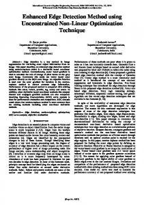
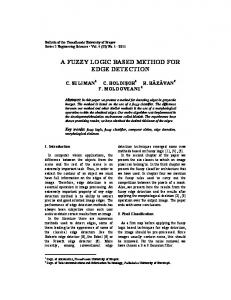
For the best configuration of the edge detection process (i.e. use the real norm and quadratic interpolation between neighbors for the NMS), we calculated the edge position bias and orientation bias mean and standard deviation (Figure 8) on the circle images. We can see that the edge position is always found inside the circle. This behavior is normal and not due to the edge detection method, as it comes from the Gaussian filtering, as shown in [1], and any smoothing operator will give the same kind of results. We compared the measured displacement with the theoretical displacement [1] and the two curves fit perfectly. The only way to avoid this error is to have a model that not only takes into account the image intensity smoothing [12], but also the local curvature or a more general shape (like a corner shape in [7]). We can also notice that the angle bias mean and standard deviation are lower than those that were found for straight edges. This is maybe due to the fact that straight edges generate more “bad” situations than curves. We present results on part of a real aerial image (Figure 9) of both the classic method and our method. We can easily see that the shape of curved features that was almost lost with the classic method is still present with our method. The brain image (Figure 10) is another example of the precision of our edge detection method. These images were taken from the database created at the SPIE Conference “Application of Artificial Intelligence X: Machine Vision and Robotics”.
5 Conclusion In this article we presented an enhancement of the Non-Maxima Suppression edge detection method which gives us the edge position at a sub-pixel accuracy. Since this method is very simple and costs only a few additions and multiplications per detected edge pixel, it can be easily implemented and incorporated in a real-time vision system, and it should be used to increase the precision and reliability of vision algorithms that use edges as input. The result we got on a wide variety of synthetic and real images are very promis1 of a pixel. ing since they show that the precision of this edge detector is less than 10 We computed the accuracy of this edge detection method in an objective manner, so that the results can be easily compared with other algorithms.
RR n˚2724
16
Fre´de´ric Devernay
Position bias mean and standard deviation (pixels)
0 real norm & quadratic interpolation -0.05 -0.1 -0.15 -0.2 -0.25 -0.3 -0.35 -0.4 -0.45 5
10
15
20
25 30 35 Circle radius (pixels)
40
45
50
Angle bias mean and standard deviation (degrees)
2 angle bias mean angle bias standard deviation
1.8 1.6 1.4 1.2 1 0.8 0.6 0.4 0.2 0 -0.2 0
5
10
15
20 25 30 Circle radius (pixels)
35
40
45
50
Figure 8: Measured edge displacement as a function of circle radius, and angle bias mean and standard deviation. We used a Gaussian filter with � = 2:0 to calculate INRIA derivatives. The displacement in the case of curved edges is not due to the edge detection method (it is due to image smoothing), and corresponds to what is predicted by the theory [1].
A NMS Method for Edge Detection with Sub-Pixel Accuracy
17
Figure 9: Results of the classic NMS algorithm (left) and of the sub-pixel approximation (right) on a 100x100 region of an aerial image. The gradient was calculated using a second order Deriche recursive filter with � = 1:2. RR n˚2724
18
Fre´de´ric Devernay
Figure 10: Result of the edge detection at sub-pixel accuracy on a 175�175 magnetic resonance image of a human brain.
INRIA
A NMS Method for Edge Detection with Sub-Pixel Accuracy
19
One advantage over existing edge refinement methods [11, 14, 15, 12] is its very low computational cost, since we only do a one-dimensional interpolation where most other methods work on two-dimensional data. Besides, other methods usually try to find a better estimate of the edge position using edge pixels that are given up to within a pixel, thus using regularization, whereas this method gets a better estimate of the edge position directly from the image intensity data. In the future, we plan to use this edge detector to calculate some higher degree differential properties of the curves such as Euclidean, affine, or even projective curvature, and we will also use it to enhance the precision of existing and future algorithms.
References [1] V. Berzins. Accuracy of laplacian edge detectors. Computer Vision, Graphics, and Image Processing, 27:195–210, 1984. [2] J. F. Canny. Finding edges and lines in images. Technical Report AI-TR-720, Massachusets Institute of Technology, Artificial Intelligence Laboratory, June 1983. [3] J. F. Canny. A computational approach to edge detection. IEEE Transactions on Pattern Analysis and Machine Intelligence, 8(6):769–798, November 1986. [4] R. Deriche. Using canny’s criteria to derive a recursively implemented optimal edge detector. The International Journal of Computer Vision, 1(2):167–187, May 1987. [5] R. Deriche. Fast algorithms for low-level vision. IEEE Transactions on Pattern Analysis and Machine Intelligence, 1(12):78–88, January 1990. [6] R. Deriche. Recursively implementing the gaussian and its derivatives. Technical Report 1893, INRIA, Unite´ de Recherche Sophia-Antipolis, 1993. [7] R. Deriche and T. Blaszka. Recovering and characterizing image features using an efficient model based approach. In Proceedings of the International Conference on Computer Vision and Pattern Recognition, pages 530–535, New-York, June 1993. IEEE Computer Society, IEEE.
RR n˚2724
20
Fre´de´ric Devernay
[8] O. D. Faugeras. Ge´ome´trie affine et projective en vision par ordinateur : I le cas des courbes. Technical report, INRIA, 1993. To appear. [9] R. M. Haralick and L. G. Shapiro. Computer and Robot Vision, volume 1. Addison-Wesley, 1992. [10] Robert Haralick. Digital step edges from zero crossing of second directional derivatives. IEEE Transactions on Pattern Analysis and Machine Intelligence, 6(1):58–68, January 1984. [11] A. Huertas and G. Medioni. Detection of intensity changes with subpixel accuracy using laplacian-gaussian masks. IEEE Transactions on Pattern Analysis and Machine Intelligence, 8(5):651–664, September 1986. [12] V. S. Nalwa and T. O. Binford. On detecting edges. IEEE Transactions on Pattern Analysis and Machine Intelligence, 8(6):699–714, 1986. [13] Jun Shen and Serge Castan. An optimal linear operator for step edge detection. CVGIP: Graphics Models and Image Processing, 54(2):112–133, March 1992. [14] Ali J. Tababai and O. Robert Mitchell. Edge location to subpixel values in digital imagery. IEEE Transactions on Pattern Analysis and Machine Intelligence, 6(2):188–201, March 1984. [15] Thierry Vie´ville and Olivier D. Faugeras. Robust and fast computation of unbiased intensity derivatives in images. In Giulio Sandini, editor, Proceedings of the 2nd ECCV, pages 203–211, Santa-Margherita, Italy, 1992. Springer-Verlag.
INRIA
Unite´ de recherche INRIA Lorraine, Technopoˆle de Nancy-Brabois, Campus scientifique, 615 rue du Jardin Botanique, BP 101, 54600 VILLERS LE`S NANCY Unite´ de recherche INRIA Rennes, Irisa, Campus universitaire de Beaulieu, 35042 RENNES Cedex Unite´ de recherche INRIA Rhoˆne-Alpes, 46 avenue Fe´lix Viallet, 38031 GRENOBLE Cedex 1 Unite´ de recherche INRIA Rocquencourt, Domaine de Voluceau, Rocquencourt, BP 105, 78153 LE CHESNAY Cedex Unite´ de recherche INRIA Sophia-Antipolis, 2004 route des Lucioles, BP 93, 06902 SOPHIA-ANTIPOLIS Cedex
E´diteur INRIA, Domaine de Voluceau, Rocquencourt, BP 105, 78153 LE CHESNAY Cedex (France) ISSN 0249-6399