A nonlinear modelling-based high-order response surface method for ...

Hydrol. Earth Syst. Sci. Discuss., doi:10.5194/hess-2016-191, 2016 Manuscript under review for journal Hydrol. Earth Syst. Sci. Published: 13 June 2016 c Author(s) 2016. CC-BY 3.0 License.

1 2

A nonlinear modelling-based high-order response surface method for predicting monthly pan evaporations

3 4

Behrooz Keshtegar*,1, Ozgur Kisi 2

5

1. Department of Civil Engineering, Faculty of Engineering, University of Zabol, P.B. 9861335856, Zabol, Iran

6

2. Department of Civil Engineering, Faculty of Architecture and Engineering, University of Canik Basari,

7

Samsun, Turkey

8 9

* Corresponding author. Tel.: 00989151924206, Fax: 00985431232074. -E-mail addresses: [email protected] (B. Keshtegar), [email protected] (O. Kisi)

1


10

Abstract: Accurate modelling of pan evaporation has a vital importance in the planning and

11

management of water resources. In this paper, the response surface method (RSM) is

12

extended for estimation of monthly pan evaporations using high-order response surface

13

(HORS) function. A HORS function is proposed to improve the accurate predictions with

14

various climatic data, which are solar radiation, air temperature, relative humidity and wind

15

speed from two stations, Antalya and Mersin, in Mediterranean Region of Turkey. The

16

HORS predictions were compared to artificial neural networks (ANNs), neuro-fuzzy

17

(ANFIS) and fuzzy genetic (FG) methods in these stations. Finally, the pan evaporation of

18

Mersin station was estimated using input data of Antalya station in terms of HORS, FG,

19

ANNs, and ANFIS modelling. Comparison results indicated that HORS models performed

20

slightly better than FG, ANN and ANFIS models. The HORS approach could be successfully

21

and simply applied to estimate the monthly pan evaporations.

22

Keywords: Evaporation; high-order response surface; fuzzy genetic; neuro-fuzzy; neural

23

network

24 25

1. Introduction

26

Evaporation is critical in water resources development and management. In arid and semi-

27

arid regions where water resources are rare, the prediction of evaporation turns out to be more

28

interesting in the planning and management of water resources (Karimi-Googhari, 2010).

29

Accurate determination evaporation amount from the soil is vital for analyzing water balance

30

at the land surface, which is essential to compute drainage requirements for preventing water

31

logging and moving away excess water from the root zone to develop crop production (de

32

Ridder and Boonstra, 1994; Kim et al., 2014). In practice, the estimation of evaporation can

33

be accomplished by direct or indirect methods. Pan evaporation (Epan) is one of the direct

34

methods for evaporation measurements. Estimation of Epan is of impressive significance to

2


35

hydrologists and agriculturists. Indirect methods, for example, mass transfer and water budget

36

techniques, taking into account meteorological data have been utilized to estimate

37

evaporation on a water body by numerous researchers (Coulomb et al., 2001; Gavin and

38

Agnew, 2004; ).

39

In the last decades, data-driven methods such as fuzzy genetic (FG), artificial neural network

40

(ANN), adaptive neuro fuzzy inference system (ANFIS) have been applied for modelling

41

Epan (Sudheer et al., 2002; Kisi, 2009; Dogan et al., 2010; Kim et al., 2013; Kisi and

42

Tombul, 2013; Malik and Kumar, 2015) and have been successfully applied in water

43

resources (Moghaddamnia et al., 2009; Amini et al., 2010; Sanikhani et al., 2012; Kisi and

44

Tombul, 2013; Liu et al. 2014; Li et al. 2015; Khan and Valeo, 2015; Xu et al., 2016).

45

Sudheer et al. (2002) used ANN in modelling Epan and compared with Stephens-Stewart

46

(SS) method. They found that two-input ANN whose inputs are air temperature and solar

47

radiation performed better than the SS. Kisi (2009) compared the accuracy of three different

48

ANN techniques in modelling daily Epan and he indicated that the muti-layer perceptron

49

(MLP) and radial basis ANN gave almost similar estimates and their accuracies were better

50

than the GRNN and SS models. Dogan et al. (2010) successfully applied ANFIS to Epan of

51

Yuvacik Dam, Turkey and compared with multiple linear regression (MLR). Shiri et al.

52

(2011) successfully estimated daily Epan using ANFIS and ANN methods. Kim et al. (2013)

53

used two different ANN, MLP and a cascade correlation neural network (CCNN), in

54

prediction of daily Epan and found CCNN to perform better than the MLP. Kisi and Tombul

55

(2013) successfully modeled Epan of Antalya and Mersin stations, Turkey by using FG and

56

compared with ANN and ANFIS methods. They found FG method to be superior to the other

57

methods in modelling Epan. Malik and Kumar (2015) modeled daily Epan of Pantnagar,

58

located in Uttarakhand, India by using co-active ANFIS, ANN and MLR methods and they

59

reported that the ANN had better accuracy than the other models in modelling Epan. The

3


60

main disadvantage of the ANFIS and ANN methods are their complex formulations.

61

Therefore, simpler and more efficient models are needed for estimating Epan in practical

62

applications.

63

The main aim of this study is to investigate the ability of high-order response surface (HORS)

64

function in estimation of Epan and compare with FG, ANFIS and ANN models previously

65

developed by Kisi and Tombul (2013). This is the first study that applies HORS in Epan

66

modelling.

67 68

2. High-order response surface method

69

In the stochastic process e.g. the pan evaporation, the accurate prediction is vital important in

70

terms of a set of several input variables, which are selected based on climatic data. Generally,

71

the evaporation is an implicit process that can be depended on several input variables (X)

72

such as air temperature, solar radiation, relative humidity and wind speed. A finding the

73

closed-form expression for evaporation based on input climatic variables is the main effort to

74

predict the availability of evaporation process because it cannot be obtained when accurate

75

approximation is not available to evaluate the evaporations. To overcome this difficulty, it

76

can be implemented the response surface methodology (RSM) to estimate the monthly pan

77

evaporation by an approximate closed-form expressions.

78

The RSM was proposed based on a set of mathematical polynomial functions through a

79

number of set experiments for increasing the computational efficiency (Bucher and Bourgund

80

1990) that it is useful for modelling and evaluating an implicit process as a response surface

81

function in explicit form. It is expressed a function E(X) based on n input variables X (x1,

82

x2,…, xn) using a second–order polynomial form with cross terms expression as follows

83

(Khuri and Cornell 1996):

84

Eˆ ( X )  a0   ai xi    aij xi x j

n

i 1

n

n

(1)

i 1 j i

4


85

In which, Eˆ ( X ) is the second–order approximated response surface function (RSF) for

86

monthly pan evaporation, n is the number of input variables such as air temperature, solar

87

radiation, relative humidity and wind speed, a0 , ai , and aij are the unknown coefficients that

88

this function has 1  n  (n  1)( n  2) / 2 coefficients to be determined based on calibration

89

of a number of set experimental samples. It may be provided an appropriate prediction for the

90

evaporation through the inclusion of the cross terms in the second-order polynomial RSF.

91

However, it may not produce accurate approximations for a highly nonlinear actual process

92

with several input variables. Therefore, a quadratic polynomial form of RSF is inappropriate

93

to approximate the pan evaporation for a wide range of stations, since the mathematical

94

nonlinear degree of the evaporation function varies for each station. It has been developed the

95

high-order response surface method by Gavin and Yau (2008) to achieve preferable

96

flexibility of RFS. The high-order RSF proposed by Gavin and Yau (2008) is more

97

inefficiently computation due to determine the order of a variable in a mixed term and use the

98

forth steps for calibration process to compute unknown coefficient. Therefore, the application

99

for predictions of evaporation is not simply based on more input variables. It is proposed a

100

high-order response surface function based on the Eq. (1) as follows:

101

Eˆ ( X )  a0   ai xi    aij xi x j    aij xi x 2j    aij xi x 3j 1 1 j i i 1 j 1 i i  i 1 j 1 2order  3order   

n

n

n

n

n

n

n

(2)

4order

102

The above RSF has 1  n  (n  1)( n  2) / 2  (Or  2)n 2 coefficients in which Or is order

103

of RSF. The main effort in the RSM form is to fit a RSF based on Eq. (2) on the limited

104

experiment points. The high-order RSF Eq. (2) is rewritten in matrix form as (Kang et al.

105

2010).

106

Eˆ ( X i )  P( X i ) T a

(3)

5


107

where, a is the coefficient vector and P( X i ) is the polynomial basic function vector at the

108

experimental point

109

P ( X )  [1, x1 , x2 ,..xn , x12 , x1 x2 , x1 x3 ,... xn2 , x13 , x1 x22 , x1 x32 ,... xn3 , x14 , x1 x23 , x1 x33 ,... xn4 ]

110

The least squares estimator is commonly used in evaluating the unknown coefficients of the

111

RSF in terms of the experimental points (Kang et al. 2010). In least square method, the

112

unknown coefficients of a are computed by minimizing the error between the experiment

113

( E ) and approximate ( Eˆ ( X ) ) data by the following matrix form

114

e( X )  [ E  P ( X ) T a ] T [ E  P ( X ) T a ]

115

In

116

experiment vector and polynomial function vector for number of data points NE ,

117

respectively.

118

The minimization of the error function in Eq. (5) with respect to the unknown coefficients of

119

a , we have e( X )  0 . Thus, the coefficients of a are yielded as follows:

120

a  [ P( X ) T P( X )] 1 [ P( X ) T E ]

121

Substituting Eq. (6) in Eq. (3), the predicted evaporation based on the high-order RSF are

122

attained as follows:

123

Eˆ ( X )  P ( X ) T [ P ( X ) T P ( X )] 1 [ P ( X ) T E ]

124

The proposed high-order polynomial RSF (2) produces more accurate results that unknown

125

coefficients are simply obtained more computationally efficient by Eq. (7). The high-order

126

RSF is obtained for predicting the pan evaporation using the set of observed points from

127

climatic data based on the a codes in MATLAB 7.10 (2010) and ran on a Intel (R) Core (TM)

128

i5 Laptop with two 2.53 GHz CPU processors and 4.0 GB RAM memory through the

129

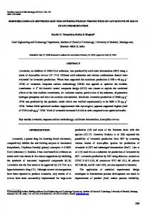
following algorithm :

X i which

is defined based on polynomial order of RSF as

which, E  [ E1 E2 E3 ... E NE ]T

(4)

(5) and P ( X )T  [ P ( X 1 ) P ( X 2 ) P ( X 3 )... P ( X NE )] are

the

a

(6)

(7)

130 6


131

Algorithm of high-order RSF:

132

Give initial parameters and database NE (Number of experiments including the train

133

and test); NV (Number of validate data); X (input train and test data); XV (input validate

134

data); E (evaporation of test and Train database).

135

Set order of RSF (2) as Or = 2, 3, or 4;

136

FOR i←1 to NE DO

137 138 139 140 141 142 143

Compute P( X i ) based on Eq. (4) END FOR Compute

the

predicted

evaporation

based

on

the

high-order

RSF

as

Eˆ ( X )  P ( X ) T [ P ( X ) T P ( X )] 1 [ P ( X ) T E ]

Determine unknown coefficients as

a  [ P( X ) T P( X )] 1 [ P( X ) T E ]

FOR i←1 to NV DO Compute P( XVi ) based on Eq. (4)

144

END FOR

145

Determine the validated evaporation using the high-order RSF as Eˆ ( XVi )  P( XVi )T a

146 147

3. Case study

148

In the applications, monthly climatic data of two automated weather stations, Antalya and

149

Mersin station operated by the Turkish Meteorological Organization (TMO) in Turkey were

150

used in the study. These data were also used by Kisi and Tombul (2013). The Mediterranean

151

Region has a Mediterranean climate characterized by warm to hot, dry summers and mild to

152

cool, wet winters. The winter temperature reaches its max. as 24 °C and in summer it may be

153

as high as 40 °C.

154

Monthly data composed of twenty years (1986-2006) of monthly values of air temperature

155

(T), solar radiation (SR), wind speed (W), relative humidity (H) and Epan. The first ten years

7


156

data (50% of the whole data) were used to train the models, the second five years data (25%

157

of the whole data) were used for testing and the remaining five years data (25% of the whole

158

data) were used for validation for each station. Detailed information about data can be

159

obtained from Kisi and Tombul (2013).

160 161

4. Comparative statistics

162

In this study, several statistical parameters were used to evaluate the performance of

163

predicted models, which were given by the following relations (Nash and Sutcliffe 1970,

164

Willmott 1981, Daren and Smith 2007).

165 166

4.1. Root mean square error (RMSE) NE

 ( Eˆ ( X i )  Ei ) 2

167

RMSE 

168

4.2. Mean absolute errors (MAE)

i 1

(8)

NE

NE

 Eˆ ( X i )  Ei

169

MAE 

170

4.3. Model efficiency factor (EF)

i 1

(9)

NE

NE

171

EF  1 

 ( Eˆ ( X i )  Ei ) 2 i 1

NE

 ( Ei  E ) 2

   EF  1

i 1

172 173

(10) 4.4. Agreement index (d)

8


NE

174

d 1

 ( Eˆ ( X i )  Ei ) 2 i 1

NE

 ( Eˆ ( X i )  E  Ei  E ) 2

0  d 1

i 1

175

(11)

176

where, NE is the number of data experiments and E is average of the observed monthly pan

177

evaporation for each station. RMSE and MAE show the average difference between predicted

178

( Eˆ ( X i ) ) and observed ( Ei ) for ith data. Of course, lower values of RMSE and MAE indicate

179

a better fit, with zero indicating a perfect prediction.

180

Efficiency factor (EF) is calculated on the basis of the relationship between the predicted and

181

observed mean deviations and it can show the correlation between the predicted and observed

182

data. EF is better suited to evaluate model goodness-of-fit than the R2, because R2 is

183

insensitive to additive and proportional differences between model prediction and

184

observations.

185

The agreement index is a descriptive measure that the range of d is similar to that of R2 and

186

varies between 0 (no correlation) and 1 (perfect fit). R2 is overly sensitive to extreme values

187

because it is sensitive to differences in the observed and predicted means and variances, the

188

factor d can be applied to overcome this difficulties based on Eq. (11) because the agreement

189

index was not designed to be a measure of correlation (Daren and Smith 2007).

190 191

5. Illustrative applications and results

192

The performance including both the accuracy and agreement of the HORS methods are

193

evaluated through two different stations such as Antalya and Mersin stations. The four

194

comparative statistics i.e. RMSE, MAE, d, and EF are used to illustrate the performance of

195

proposed HORS functions and the performance of HORS functions are compared with the

196

FG, ANFIS, and ANN models in three applications. In the first application, pan evaporations

9


197

of were separately calibrated based on climatic input data for each station. In the second

198

application, the Mersin’s pan evaporations were estimated using data from Antalya stations.

199

In the third application, the Mersin’s pan evaporations were approximated using input

200

climatic data from both Antalya and Mersin stations. For this three applications, the

201

comparative results of three order RSFs including 2-order, 3-order, and 4-order are

202

determined and compared with the soft computing–based FG, ANFIS, ANN models. A

203

program code was developed by MATLAB language for HORS models based on algorithm

204

of high-order RSF. The results of FG, ANFIS and ANN models were obtained from the study

205

of Kisi and Tombul (2013).

206 207

5.1. Predicting monthly pan evaporations of Antalya and Mersin stations

208

In the present paper, three different HORS models including 2-order RSF which indicates a

209

response surface function with second–order polynomial form, 3-order RSF, and 4-order RSF

210

were developed for predicting the monthly pan evaporations based on four inputs, T, SR, W

211

and H for Antalya and Mersin stations. The test and validation results of each model are

212

tabulated and compared with FG, ANFIS and ANN in Table 1. In the table, the

213

FG(2,gauss,100000) model represents a FG model comprising 2, 2, 2 and 2 Gaussian MFs for

214

each climatic input and 100000 iterations. ANFIS(2,gauss,10) model represents an ANFIS

215

model including 2, 2, 2 and 2 Gaussian MFs for each input and 10 iterations and ANN(4,1,1)

216

model indicates an ANN model having 4, 1 and 1 nodes for the input, hidden and output

217

nodes, respectively. In Antalya Station, RSF models perform superior to the FG, ANFIS and

218

ANN models in both test and validation periods. The accuracy of the FG model with respect

219

to RMSE, MAE, EF and d were improved by 69%, 82%, 10% and 3% using 4-order RFS,

220

respectively. In Mersin Station, also the RSF models have better accuracy than the soft

221

computing techniques from the RMSE, MAE, EF and d viewpoints. The 4-order RFS

10


222

improved the accuracy of the FG model with respect to RMSE, MAE, EF and d by 176%,

223

202%, 7.2% and 44%, respectively. Figures 1-2 illustrates the estimates of the FG, ANFIS,

224

ANN and RFS models in validation stage for the Antalya and Mersin stations, respectively. It

225

is apparent from the fit line equations and R2 values that the RFS models have less scattered

226

estimates which are closer to the ideal line than those of the soft computing models. 3-order

227

and 4-order RSF models have almost similar accuracy and they are slightly better than the 2-

228

order RSF models.

229

period are: 4-order RFS, 3-order RFS, 2-order RFS, FG, ANFIS and ANN.

230

Table 2 reports the total pan evaporation (TPA) predictions of each model. As clearly

231

observed from the table that the RFS models estimate TPA better than the soft computing

232

methods. Among the RFS methods, 4-order RFS provides the closest estimate for both

233

stations in the validation stage. For the Antalya Station, the observed TPA of 322 mm was

234

estimated as 306 mm by 4-order RFS with an underestimation of 4.8% while it was

235

respectively estimated as 303, 302, 283, 275 and 275 mm by 3-order RFS, 2-order RFS, FG,

236

ANFIS and ANN models with underestimations of 5.7, 6.1, 12, 14.5 and 15.3%. For the

237

Mersin Station, while the 4-order RFS estimated the TPA as 179 mm, compared to the

238

measured 173 mm, with an overestimation of 3.5% in the validation period, the 3-order RFS,

239

2-order RFS, FG, ANFIS and ANN models resulted in 180, 186, 216, 225 and 230 mm, with

240

overestimations of 4, 7.4, 25, 30 and 33%, respectively.

In both stations, the accuracy ranks of the applied models in validation

241 242

5.2. Predicting Mersin’s pan evaporations using climatic data of Antalya

243

In this section of the study, the accuracy of RFS models was tested in prediction of Mersin’s

244

Epan using climatic input data of Antalya Station and results were compared with soft

245

computing methods. The validation results of the applied models are given in Table 3. It is

246

apparent from the table that the RFS models perform superior to the FG, ANFIS and ANN

11


247

models in terms of RMSE, MAE, EF and d. The RMSE accuracies of the FG, ANFIS and

248

ANN models were increased by 110, 132 and 133% using 4-order RFS, separately. The worst

249

2-order RFS increased the MAE, EF and d accuracies of the best soft computing FG model

250

by 67, 224 and 32%, respectively. The TPA predictions are also compared in Table 3. Similar

251

to the previous applications, here also the RFS models outperform the soft computing

252

methods. 4-order RFS estimated the TPA as 176 mm, instead of measured 173 mm, with an

253

overestimation of 1.8% in the validation period, 3-order RFS, 2-order RFS, FG, ANFIS and

254

ANN resulted in 178, 184, 205, 215 and 212 mm, with overestimations of 2.6, 6.4, 18.2, 24.1

255

and 22.7%, respectively. There is a slight difference between RFS models. Figure 3 compares

256

the Epan estimates of each model with the corresponding observed values in validation stage.

257

It is obvious that the RFS model has less scattered estimates and they are closer to the ideal

258

line than those of the soft computing methods. It can be said that the RFS models can be

259

successfully used in estimation of Epan without local input data.

260 261

5.3. Predicting Mersin’s pan evaporations using climatic data of Antalya and Mersin

262

In this section of the study, the RFS models are compared with soft computing methods in

263

Epan estimation using local and external inputs. Climatic input data of Mersin and Antalya

264

stations were used as inputs to the applied models to estimate Epan of Mersin Station.

265

Limited climatic inputs were also considered as inputs to the models in this part of the study.

266

Estimating Epan using limited input variables is very essential especially for the developing

267

countries where wind speed and relative humidity data are missing or unavailable. The

268

validation results of the RFS and soft computing methods are provided in Table 4. The

269

superior accuracy of the RFS models to the soft computing methods are clearly seen from the

270

table. In case four-input parameter, 4-order RFS1 increased accuracy of the FG1 by 316, 371,

271

7.3 and 43% in terms of RMSE, MAE, EF and d, respectively. Furthermore, the RMSE

272

accuracies of the two-input FG2, ANFIS2 and ANN2 models were increased by 143, 243, 12


273

158 and 54 using the 4-order RFS2 model with two inputs. RFS models seem to be more

274

successful than the soft computing models in estimating TPA values in validation stage. The

275

scatterplots of the estimates obtained from RFS and soft computing models in validation

276

stage are demonstrated in Figures 4 and 5 for the four- and two-input models. In both cases,

277

4-order and 3-order RFS models have similar estimates and they are closer to the observed

278

Epan values than those of the other models. Comparison of two- and four-input models

279

indicates that the wind speed and relative humidity variables are very effective on Epan and

280

removing these inputs significantly decreases models’ accuracies especially for the RFS

281

models.

282 283 284

6. Conclusions

285

The present study investigated the ability of response surface method to predict the monthly

286

pan evaporations. A high-order response surface (HORS) function was proposed with simple

287

formulation to estimate the pan evaporations using climatic input variables including air

288

temperature (T), relative humidity (H), wind speed (W) and solar radiation (SR) for Antalya

289

and Mersin stations. The HORS function was extended based on order of polynomial

290

functions based on input variables more than two. In this approach, the high-order

291

polynomial functions are simply and directly calibrated based on the observed climatic data

292

and relative experiments of evaporation data for each station. The accuracy of HORS

293

function with second-order, third-order and four-order were compared to the FG, ANFIS,

294

ANN approaches for estimating the monthly pan evaporations using several comparative

295

statistics such as root mean square error (RMSE), mean absolute errors (MAE), model

296

efficiency factor (EF), and agreement index (d). Three applications of HORS function were

297

compared with the soft computing–based models based on input variables of Antalya and

298

Mersin stations. In the first stage of the predictions, the performance of proposed HORS

13


299

models was compared in estimating pan evaporations of Antalya and Mersin stations,

300

separately. In the second application, the prediction results of HORS functions for

301

evaporation of Mersin station with input variables of Antalya were compared.

302

In the third part of the study, models of HORS and FG, ANFIS, and ANN were compared

303

with each other in estimating Mersin’s pan evaporations using input data of the Antalya and

304

Mersin stations. Comparison of the models indicated that the 4-order RSF models generally

305

performed better than the 2-order RSF, 3-order RSF, FG, ANFIS and ANN models. The

306

RSFs with second, third and fourth-order polynomial functions were performed better than

307

the soft computing-based models inclining both the accuracy (less RMSE and MAE than FG,

308

ANFIS, ANN) and agreement (more EF and d than FG, ANFIS, ANN). This result revealed

309

that the HORS models were much simpler than the other models and could be successfully

310

used in estimating monthly pan evaporations. The 3-order RSF and 4-order RSF models

311

provided the closest total pan evaporation estimates based on RMSE for Antalya and Mersin

312

stations in the validation period, respectively. The comparative statistics for both stations

313

were computed similar based on 3-order RSF and 4-order RSF models.

314 315

References

316

Amini, M., Abbaspour, K.C., Johnson, C.A. (2010). A comparison of different rule-based

317

statistical models for modelling geogenic groundwater contamination, Environmental

318

Modelling & Software, 25(12): 1650-1657.

319 320

Bucher, C.G., Bourgund, U. 1990. A fast and efficient response surface approach for structural reliability problems. Structural Safety,7(1):57-66.

321

Chang, F-J, Chang, L-C, Kao, H-S, Wu, G-R, 2010. Assessing the effort of meteorological

322

variables for evaporation estimation by self-organizing map neural network, Journal of

323

Hydrology, 384, 118–129.

14


324

Coulomb, C.V., Legessea, D., Gassea, F., Travic, Y., Chernetd, T., 2001. Lake evaporation

325

estimates in tropical Africa (Lake Ziway, Ethiopia). Hydrological Processes 245 (1–4),

326

1–18.

327

Daren Harmel, R., Smith, P.K., 2007. Consideration of measurement uncertainty in the

328

evaluation of goodness-of-fit in hydrologic and water quality modelling, Journal of

329

Hydrology, 337: 326– 336.

330

de Ridder, N. and Boonstra, J., 1994. Analysis of water balances. In: Ritzema HP (ed)

331

Drainage principles and applications, 2nd edn, International Institute for Land

332

Reclamation and Improvement (ILRI). Wageningen, The Netherlands: 601–633.Nash,

333

J.E., Sutcliffe, J.V., 1970.

334

Dogan, E., Gumrukcuoglu, M., Sandalci, M., Opan, M., 2010. Modelling of evaporation from

335

the reservoir of Yuvacik dam using adaptive neuro-fuzzy inference systems, Engineering

336

Applications of Artificial Intelligence, 23, 961–967.

337 338 339 340

Gavin, H., Agnew, C.A., 2004. Modelling actual, reference and equilibrium evaporation from a temperate wet grassland. Hydrological Processes 18 (2), 229–246. Gavin, H.P., Yau, S.C., 2008. High-order limit state functions in the response surface method for structural reliability analysis. Structural Safety, 30:162–179.

341

Kang, H.M., Choo, J.F., 2010. An efficient response surface method using moving least

342

squares approximation for structural reliability analysis, Probabilistic Engineering

343

Mechanics, 25: 365-371.

344 345 346 347

Karimi-Googhari, S., 2010. Daily Pan Evaporation Estimation Using a Neuro-Fuzzy-Based Model. Trends in Agricultural Engineering, 2010: 191-195. Khan, U. T. and Valeo, C., 2015. Dissolved oxygen prediction using a possibility-theory based fuzzy neural network, Hydrol. Earth Syst. Sci. Discuss., 12, 12311-12376.

15


348 349

Khuri, A.I., Cornell, J.A., 1996. Response surfaces designs and analyses. 2nd ed. Marcel Dekker.

350

Kim, S., Singh, V.P. and Seo, Y., 2014. Evaluation of pan evaporation modelling with two

351

different neural networks and weather station data. Theoretical and Applied Climatology,

352

117(1-2): 1-13.

353

Kim, S., Singh, V.P., Seo, Y., 2013. Evaluation of pan evaporation modelling with two

354

different neural networks and weather station data, Theoretical and Applied Climatology,

355

117 (1), 1-13.

356 357 358 359

Kisi, O., 2009. Daily pan evaporation modelling using multi-layer perceptrons and radial basis neural networks, Hydrol. Process., 23, 213–223. Kisi, O., Tombul, M., 2013., Modelling monthly pan evaporations using fuzzy genetic approach, Journal of Hydrology 477:203–212.

360

Li, X., Maier, H. R., Zecchin, A. C. (2015). Improved PMI-based input variable selection

361

approach for artificial neural network and other data driven environmental and water

362

resource models. Environmental Modelling & Software, 65, 15–29.

363

Liu, K.K., Li, C.H., Cai, Y.P., Xu, M., and Xia, X.H., 2014. Comprehensive evaluation of

364

water resources security in the Yellow River basin based on a fuzzy multi-attribute

365

decision analysis approach, Hydrol. Earth Syst. Sci., 18, 1605-1623.

366

Malik, A., Kumar, A. 2015., Pan Evaporation Simulation Based on Daily Meteorological

367

Data Using Soft Computing Techniques and Multiple Linear Regression, Water Resour

368

Manage, 29: 1859–1872.

369

MATLAB version 7.10.0. 2010. Natick, Massachusetts: The Math Works Inc.

370

Moghaddamnia, A., Gousheh, M.G., Piri, J., Amin, S. and Han, D., (2009). Evaporation

371

estimation using artificial neural networks and adaptive neuro-fuzzy inference system

372

techniques. Advances in Water Resources, 32(1): 88-97.

16


373 374

Nash JE, Sutcliffe JV (1970) River flow forecasting through conceptual models, Part I: a discussion of principles. Journal of Hydrology, 10 (3): 282–290.

375

Sanikhani, H., Kisi, O., Nikpour, M.R. and Dinpashoh, Y., (2012). Estimation of Daily Pan

376

Evaporation Using Two Different Adaptive Neuro-Fuzzy Computing Techniques. Water

377

Resources Management, 26(15): 4347-4365.

378

Shiri, J., Dierickx, W., Baba, A. P-A, Neamati, S., Ghorbani, M.A. 2011., Estimating daily

379

pan evaporation from climatic data of the State of Illinois, USA using adaptive neuro-

380

fuzzy inference system (ANFIS) and artificial neural network (ANN), Hydrologic

381

Research, 42 (6) 491-502

382 383 384

Sudheer K.P., Gosain A.K., Rangan D.M., Saheb S.M., 2002. Modelling evaporation using an artificial neural network algorithm. Hydrological Processes 16: 3189–3202. Xu, J., Chen, Y., Bai, L., and Xu, Y., 2016. A hybrid model to simulate the annual runoff of

385

the Kaidu River in northwest China, Hydrol. Earth Syst. Sci., 20, 1447-1457.

386

Willmott, C.J. 1981. On the validation of models. Phys. Geograph. 2(2): 184-194.

387

17


388

Table 1. Error statistics for each model in test and validation stage. Model

Structure

RMSE (mm)

Test MAE EF (mm) Antalya

FG

(2,gauss,100000)

0.942

0.699

0.888

0.968

1.055 0.875 0.855 0.956

ANFIS

(2,gauss,10)

0.964

0.719

0.883

0.966

1.152 0.964 0.827 0.950

d

RMSE (mm)

Validation MAE (mm)

EF

d

ANN

(4,1,1)

0.931

0.716

0.891

0.970

1.179 0.978 0.819 0.947

2-order RSF

Second –order

0.733

0.550

0.932

0.981

0.725 0.551 0.932 0.981

3-order RSF

Third –order

0.667

0.500

0.944

0.985

0.650 0.481 0.945 0.985

4-order RSF

Fourth –order

0.585

0.441

0.957

0.988

0.626 0.480 0.949 0.986

Mersin FG

(3,gauss,50000)

1.328

1.114

0.050

0.841

0.926

0.775

0.914

0.526

ANFIS

(2,gauss,100)

1.461

1.252

-0.150 0.816

1.100

0.925

0.887

0.332

ANN

(4,1,1)

1.528

1.340

-0.256 0.805

1.176

1.026

0.875

0.235

2-order RSF

second –order

0.878

0.714

0.585

0.913

0.416

0.341

0.978

0.904

3-order RSF

Third –order

0.779

0.582

0.673

0.930

0.335

0.260

0.985

0.938

4-order RSF Fourth –order 0.735 0.549 0.709 0.937 0.336 0.257 0.985 0.938 Note that the test and validation results of the FG, ANFIS and ANN models were obtained from Kisi and Tombul (2013)

18


Table 2. Total pan evaporation estimates - test and validation period. Total pan evaporation (mm)

Relative error (%)

Test

Validation

Test

Validation

Observed

333

322

-

-

FG

309

283

-7.2

-12.0

ANFIS

303

275

-8.8

-14.5

ANN

301

272

-9.6

-15.3

2-order RSF

316

302

-5.0

-6.1

3-order RSF

319

303

-4.3

-5.7

4-order RSF

321

306

-3.5

-4.8

Observed

171

173

-

-

FG

233

216

36.5

24.7

ANFIS

241

225

41.0

29.8

ANN

246

230

44.0

33.1

2-order RSF

207

186

21.2

7.4

3-order RSF

201

180

17.7

4

4-order RSF

198

179

16.0

3.5

Antalya Station

Mersin Station

Note that the validation results of the FG, ANFIS and ANN models were obtained from Kisi and Tombul (2013)

19


Table 3. Comparison of models in estimating Mersin's pan evaporation using the climatic data of Antalya in validation period. Model

Structure

RMSE (mm)

MAE (mm)

EF

d

Total pan evaporation (mm)

Relative error (%)

FG

(3,gauss,100000)

0.773

0.631

0.940

0.670

205

18.2

ANFIS

(2,gauss,100)

0.853

0.719

0.920

0.598

215

24.1

ANN

(4,1,1)

0.859

0.713

0.926

0.592

212

22.7

2-order RSF

Second –order

0.377

0.290

0.981

0.922

184

6.4

3-order RSF

Third –order

0.373

0.275

0.982

0.923

178

2.6

4-order RSF

Fourth –order

0.368

0.288

0.982

0.925

176

1.8

Note that the validation results of the FG, ANFIS and ANN models were obtained from Kisi and Tombul (2013)

20


Table 4.Comparison of models in estimating Mersin's pan evaporation using the climatic data of Antalya and Mersin in validation period. Model

Structure

RMSE (mm)

MAE (mm)

EF

d

Total pan evaporation (mm)

Relative error (%)

Mersin using the climatic data of TA, SRA, WA, HA, TM, SRM, WM and HM FG1

(2,gauss,100000)

0.896

0.735

0.921

0.556

211

22.0

ANFIS1

(2,gauss,500)

1.047

0.869

0.901

0.394

220

26.9

ANN1

(8,1,1)

1.043

0.884

0.898

0.398

222

28.4

2-order RSF1

Second –order

0.345

0.286

0.984

0.934

178

2.8

3-order RSF1

Third –order

0.249

0.195

0.992

0.966

174

0.5

4-order RSF1

Fourth –order

0.215

0.156

0.994

0.975

174

0.7

Mersin using the climatic data of TA, SRA, TM, and SRM FG2

(3,gauss,10000)

0.995

0.846

0.904

0.416

220

27.0

ANFIS2

(2,gauss,100)

1.402

1.096

0.845

-0.087

212

22.4

ANN2

(4,1,1)

1.055

0.922

0.895

0.385

225

29.8

2-order RSF2

second –order

0.638

0.505

0.956

0.775

198

14.5

3-order RSF2

Third –order

0.412

0.345

0.978

0.906

190

9.2

4-order RSF2 Fourth –order 0.409 0.338 0.978 0.908 188 8.8 Note that the validation results of the FG, ANFIS and ANN models were obtained from Kisi and Tombul (2013)

21


Figures

Fig. 1. The observed and estimated pan evaporation of the Antalya Station in validation period (The results of FG, ANFIS and ANN were obtained from Kisi and Tombul (2013)).

22


Fig. 2. The observed and estimated pan evaporation of the Mersin Station in validation period (The results of FG, ANFIS and ANN were obtained from Kisi and Tombul (2013)).

23


Fig. 3. The observed and estimated pan evaporation of the Mersin Station using the climatic data of Antalya Station in validation period (The results of FG, ANFIS and ANN were obtained from Kisi and Tombul (2013)).

24


Fig. 4. The observed and estimated pan evaporation of the Mersin Station using the climatic data of Antalya and Mersin stations (i.e. TA, SRA, WA, HA, TM, SRM, WM and HM) in validation period (The results of FG, ANFIS and ANN were obtained from Kisi and Tombul (2013)).

25


Fig. 5. The observed and estimated pan evaporation of the Mersin Station using the climatic data of Antalya and Mersin stations (i.e. TA, SRA, TM, and SRM) in validation period (The results of FG, ANFIS and ANN were obtained from Kisi and Tombul (2013)). 389

26

A nonlinear modelling-based high-order response surface method for ...

A nonlinear modelling-based high-order response surface method for ...

Suggest Documents

A Highorder extended finite element method for ...

A method for measuring the nonlinear response in dielectric

Comparison between Taguchi Method and Response Surface ...

Finite element analysis and response surface method

Review on Application of Response Surface Method

The Response Surface Method Applied to Deep

Comparison between Taguchi Method and Response Surface ...

Distributed Collaborative Response Surface Method ... - Springer Link

RESPONSE SURFACE METHODOLOGY FOR

A method for solving nonlinear Volterra's

A New Iterative Method for Solving Nonlinear

A COLLOCATION METHOD FOR SOLVING NONLINEAR VOLTERRA ...

A new method for solving nonlinear fractional

A Wavelet Method for Solving Nonlinear Time

Response surface method for assessing energy ... - Semantic Scholar

An improved response surface method for reliability ...

Response surface method for assessing energy production from ...

Application of Response Surface Method for Preparation, Optimization

Use of response surface method for maximizing the ... - CyberLeninka

An improved response surface method for reliability ... - Techno Press

A New Method Based on TOPSIS and Response Surface Method for

A Continuum Method for Modeling Surface Tension

A Cutting Surface Method for Uncertain Linear

a surface definition method for an interfacial