Structural Engineering and Mechanics, Vol. 42, No. 2 (2012) 175-189
175
DOI: http://dx.doi.org/10.12989/sem.2012.42.2.175
An improved response surface method for reliability analysis of structures Hasan Basri Basaga*1, Alemdar Bayraktar1a and Irfan Kaymaz2b 1
Department of Civil Engineering, Karadeniz Technical University, 61080, Trabzon, Turkey 2 Department of Mechanical Engineering, Ataturk University, 25240, Erzurum, Turkey
(Received December 17, 2010, Revised February 22, 2012, Accepted March 13, 2012) Abstract. This paper presents an algorithm for structural reliability with the response surface method. For this aim, an approach with three stages is proposed named as improved response surface method. In the algorithm, firstly, a quadratic approximate function is formed and design point is determined with First Order Reliability Method. Secondly, a point close to the exact limit state function is searched using the design point. Lastly, vector projected method is used to generate the sample points and Second Order Reliability Method is performed to obtain reliability index and probability of failure. Five numerical examples are selected to illustrate the proposed algorithm. The limit state functions of three examples (cantilever beam, highly nonlinear limit state function and dynamic response of an oscillator) are defined explicitly and the others (frame and truss structures) are defined implicitly. ANSYS finite element program is utilized to obtain the response of the structures which are needed in the reliability analysis of implicit limit state functions. The results (reliability index, probability of failure and limit state function evaluations) obtained from the improved response surface are compared with those of Monte Carlo Simulation, First Order Reliability Method, Second Order Reliability Method and Classical Response Surface Method. According to the results, proposed algorithm gives better results for both reliability index and limit state function evaluations. Keywords: response surface method; structural reliability; vector projected method
1. Introduction The reliability analysis of structures deals with the calculation of the failure probability under a defined limit state conditions. The failure probability of a structural component with respect to a single failure mode can be formally calculated from (Thoft-Christensen and Baker 1982, Ayyub and McCuen 1997, Melchers 1999) pf =
∫
fX ( x ) dx
(1)
g (x ) < 0
where X is the vector of basic random variables and g(x) is the limit state (or failure) function for *Corresponding author, Ph.D., E-mail:
[email protected] a E-mail:
[email protected] b E-mail:
[email protected]
176
Hasan Basri Basaga, Alemdar Bayraktar and Irfan Kaymaz
the failure mode considered, fX(x) is the joint probability density function of the vector X. If g(x) < 0, then the failure domain, if g(x) > 0, then the safe domain and if g(x) = 0, then the failure surface are defined. The basic random variables comprise physical variables describing uncertainties in loads, material properties, geometrical data and calculation modeling. The structural safety is calculated by different reliability methods in 3 levels. Level I methods, in which uncertain parameters are modeled by one characteristic value, check the structural safety deterministically instead of computing the probability of failure explicitly. Level II methods, First Order Reliability Method (FORM) and Second Order Reliability Method (SORM), compute the probability of failure by means of approximations of the Limit State Function (LSF) at design point. The Level III methods such as Monte Carlo Simulation (MCS) and Numerical Integration compute the exact probability of failure of the whole structural system, or structural components, using the exact probability density function of all random variables. MCS needs much computational time, especially for low probability of failure, so several variance reduction techniques have been proposed, e.g. importance sampling (Melchers 1990, Bucher 1988, Zheng et al. 1991), directional simulation (Bjerager 1988), conditional expectation (Ayyub and Chia 1992), etc. Besides, the approximate methods such as FORM and SORM are not suitable for the LSF which is implicitly defined or nonlinear in normal space (Melchers 1999). The Response Surface Method (RSM) (Faravelli 1989, Bucher and Bourgund 1990) appeared an alternative method to get the reliability of structures approximately. Several researchers used the RSM in the reliability analysis with different approximations. Rajashekhar and Ellingwood (1993) proposed an adaptive procedure to develop response surface for structural reliability. The procedure was repeated until the convergence parameter defined as the distance between the center point and minimum norm point became very small or zero. Kim and Na (1997) presented an improved sequential response method. The method used the linear type response surface functions in conjunction with Rackwitz-Fiessler algorithm with the gradient projection method. An iterative solution was performed till a convergence criterion on the reliability index is satisfied. Das and Zheng (2000) examined an improve response surface method which was formed in a cumulative manner. In the algorithm, sampling points were selected by using vector projected, then the linear response surface was improved by adding square terms and lastly, the response surface function was checked until finding the satisfactory function. Zheng and Das (2000) improved the cumulative formation of response surface method and used it in the calculation of the stiffened plate safety. Gayton et al. (2003) studied a special RSM named Complete Quadratic Response Surface with ReSampling (CQ2RS) to calculate the reliability problems using a statistical formulation of the RSM problem and considering the estimate of the coordinates of a design point in the U space as a random variable, through successive experimental designs. Gomes and Awruch (2004) performed a study of reliability analysis using RSM and Artificial Neural Network techniques. It was emphasized that two techniques might turn feasible the evaluation of the structural reliability through simulation techniques. Kaymaz and McMahon (2005) proposed a new response surface method using weighted regression method instead of normal regression. This approach named ADAPRES gave good results by having selected experimental points close to the LSF. Wong et al. (2005) investigated an adaptive design approach which was presented to overcome the divergence resulted from the non-smoothness of the response surface and unrealistic design point when the loading was applied in sequence in the non-linear finite element analysis. Lee and Kwak (2006) presented a response surface method which was built by axial experimental points instead of full factorial design of experiment using with the moment method. The probability of
An improved response surface method for reliability analysis of structures
177
failure was calculated using the Pearson system and the four statistical moments obtained from the experimental data complemented by the response surface. Gavin and Yau (2008) showed a method using higher order polynomials in the response surface method instead of quadratic polynomials. The orthogonal polynomials were utilized to overcome the problems associated with ill-conditioned systems of equation. Chen et al. (2010) presented an improved response surface method based on weighted regression for the anti-slide reliability analysis of concrete gravity dam. It was emphasized that this algorithm is saved the arithmetic operations and is enhanced the calculation efficiency and the storage efficiency. Kang et al. (2010), proposed adaptive response surface method based on moving least squares (MLS) approximation to overcome the large errors in the calculations and time consuming. The MLS approximation gave higher weight to the experimental points closer to the most probable failure point, which allows the response surface function to be closer to the limit state function at the probable failure point. In the literature, it is observed that some of the RSM methods are based on the iterative solution, some of them are based on Neural Network techniques, and some of them are based on the special algorithms. Especially, Neural Network and iterative solution required much LSF evaluations. This leads much computational time when the limit state function is defined implicitly. Besides, some researches do not give the LSF evaluations, so it does not understand if the algorithm is efficient or not. In this study, it is aimed to get the optimum solutions (minimum LSF evaluations and more accurate result) for the reliability analysis with an improved response surface method. This approach combines the Bucher and Bourgund’s (1990) algorithm and vector projected sampling (Kim and Na 1997) with a special interface algorithm.
2. Response surface method Response surface methodology (RSM) is a collection of mathematical and statistical techniques that are useful for the modeling and analysis of problems in which a response of interest is influenced by several variables and the aim is to optimize this response. In this way, the actual limit state function g(X) is replaced by a polynomial type of function gˆ ( X ) , as an example, a quadratic polynomial with cross terms (Myers 1971) n
n
i=1
i=1
n–1
2 gˆ ( X ) = a + ∑ bi x i + ∑ c i xi + ∑
n
∑
dij x i xj + ε
(2)
i = 1j = i + 1
where a, bi, ci and dij are the coefficients of the polynomial, n is the number of the variables X and ε is the random error that contains the error due to neglecting the higher order terms. In practice, it is suggested that polynomials are up to second order for the response function, often without the mixed terms because they are uneconomic for problems involving large numbers of random variables. So, Eq. (2) becomes n
n
i=1
i=1
2 gˆ ( X ) = a + ∑ bi xi + ∑ ci xi + ε
(3)
To obtain 2n + 1 unknown coefficients (a, bi, ci), the experimental points should be chosen. Bucher and Bourgund (1990) selected these points along the coordinate axis xi around the mean values of the random variables. The values of experimental points are calculated as
178
Hasan Basri Basaga, Alemdar Bayraktar and Irfan Kaymaz
− kσ i xi = µi +
(4)
in which k is an arbitrary factor (in general selected as 3), µ i and σi are the mean and standard deviation of xi respectively. The coefficients are achieved by using the least square method as (Myers 1971) –1
coeff = ( W′W ) W′g
(5)
where coeff is the coefficient vector, W indicates the design matrix including the experimental points and g represents the response vector obtained from the LSF corresponding to the experimental points. The design point is obtained from the approximate function, gˆ ( X ) , and new centre point is determined by (Bucher and Bourgund 1990) g(µ ) XM = µ + ( XD – µ ) -----------------------------g ( µ ) – g ( XD )
(6)
where XM and XD represent the centre point and the design point, respectively. This new centre point is used to obtain the second approximate function, g˜ ( X ) . 3. Improved Response Surface Method (IMPRES) algorithm The improved response surface method (IMPRES) algorithm (Baçsago a 2009) proposed in this study includes 3 stages. The first stage includes classical response surface with a quadratic approximate function which is used to obtain the design point. In the second stage, a point is searched close to the exact LSF using design point obtained in the first stage. Lastly, the vector projection technique (Kim and Na 1997) is utilized to generate the experimental points nearby the exact LSF using the point obtained previous stage. The details about the stages are given below. 3.1 The first stage of IMPRES The aim of first stage is to obtain the design point through the quadratic approximate function formed by RSM. In this stage, 2n + 1 LSF evaluations are performed. The steps of the first stage are as follows: 1. Determine the random variables, their statistical properties and implicit LSF. 2. Select the experimental points as they are seen in Fig. 1(a). (Eq. (4)). 3. Run g(X) for these experimental points. 4. Calculate 2n + 1 coefficient for the quadratic approximate function with the least square regression (Eq. (5)). 5. Apply the FORM to obtain the design point (XD) given in Fig. 1(b). 3.2 The second stage of IMPRES In this stage, it is intended to attain a point close to the exact LSF. Selecting this point requires n + 9 LSF evaluations.
An improved response surface method for reliability analysis of structures
179
Fig. 1 The first stage of the proposed algorithm
This stage includes the following steps: 1. Get the response for XD from g(X). 2. Determine the corner points (Fig. 2(a)) around the design point ( XD − + 3σ ). 3. Find the corner point whose response at g(X) is opposite sign of that obtained from step 1. In this way, two points are obtained at two different regions of the exact LSF. 4. Determine the direction (Fig. 2(b)) between the selected corner point and the design point. This direction often cuts the exact LSF. 5. Find the point (XC) which is close to the exact LSF through the direction obtained from step 4. For this purpose, firstly, a point is selected in the middle of the corner point and XD through the direction. Thus, the locations of the three points are determined. Among these, two points which are the closest to the exact LSF are selected. And also the exact LSF is located between the selected points. Five points are obtained by this procedure. Finally, the closest point to the exact LSF is selected from five points. In Fig. 2(c), two steps for the point selecting procedure is given.
Fig. 2 The second stage of the proposed algorithm
180
Hasan Basri Basaga, Alemdar Bayraktar and Irfan Kaymaz
3.3 The third stage of IMPRES Last stage includes the vector projection technique (Kim and Na 1997). This method is used to select the experimental points around the XC. For this purpose, 5n + 2 or 7n + 2 LSF evaluations are performed according to the value of f. This stage algorithm is as follows: 1. Select f = 1 and determine a set of sampling point around the XC (Eq. (7)). iT
i
xs = Xc ± f ⋅ σi ⋅ n – 1 ⋅ ε ⋅ δ
i
(7)
where • i = 1, 2, …, n …
⎧ ε1 ⎫ ⎪ ⎪ ⎧ εk = 1.0 for • ε = ⎨ ⎬⇒⎨ ⎪ ⎪ ⎩ εk = 0.9 for ⎩ εk ⎭ i
k=i
( k = 1, 2, …, n )
k≠i
(8)
i
• δ is the projected unit vector and computed for each random variable as i
hj i δ j = -------------------n i ∑ ( hk )
(9)
k=1
• in which for ith random variable ( j = 1, 2, …, n ) and hi is defined as i
i
T
i
h = u – ∆g ⋅ ( ∆g ⋅ u )
(10) i
where ∆g is the gradient vector of the exact LSF at XC and uj is equal to the Kronecker delta. The experimental points selected by vector projected method are demonstrated in Fig. 3(a).
Fig. 3 The third stage of the proposed algorithm
An improved response surface method for reliability analysis of structures
181
2. Form quadratic approximate function ( g˜ ( X ) ) and calculate the coefficients with regression analysis (Fig. 3(b)). 3. Apply the SORM to obtain the reliability index (β1). 4. Select f = 1.5 and repeat step 2 and 3 to obtain reliability index (β1.5). β1 – β1.5 5. Calculate ∇ = -------------------n–1 ⎧f = 1 6. Select f ⇒ ⎨ ⎩ f = 1.2
if if
∇ ≤ 0.03 0.03 < ∇
7. If f = 1, use step 3 results; otherwise, repeat step 2 and 3 for f = 1.2.
4. Numerical examples To illustrate the proposed approach, 5 numerical examples taken from the literature are presented. They are a uniform loaded cantilever beam (Rajashekhar and Ellingwood 1993, Gomes and Awruch 2004), a highly nonlinear LSF (Kaymaz and McMahon 2005), dynamic response of an oscillator (Bucher and Bourgund 1990, Rajashekhar and Ellingwood 1993, Gayton et al. 2003), a frame structure (Kim and Na 1997) and a truss structure (Kim and Na 1997, Lee and Kwak 2006). ANSYS (2007) finite element analysis program is used to obtain the response of frame and truss structures. For this purpose, ANSYS and the proposed algorithm is combined to perform the reliability analysis. A linear response surface function is used at the first stage of the classic RSM. The results (reliability index, probability of failure and LSF evaluations) are compared with those obtained from MCS, FORM, SORM and classic RSM. 4.1 Example 1 : Cantilever beam A uniform loaded cantilever beam with a rectangular cross section (Rajashekhar and Ellingwood 1993, Gomes and Awruch 2004) is selected as the first example. The maximum vertical displacement located at the free end of the beam is compared with the serviceability limit which is l/325 (l: length of the beam). The LSF is defined explicitly as 4
l wbl f = --------- – -----------325 8EI
(11)
where w, b, E and I are respectively uniform load per unit area, the width of the beam, modulus of elasticity and the momentum of inertia. E and l are considered as deterministic with the values of 2.6E10 N/m2 and 6 m. The load per unit area (x1) and height of the beam (x2) are selected as random variables, the statistical distributions of which are given in Table 1. In light of this information, the LSF becomes –8 x h = 0.01846154 – 7.476923077 × 10 ----13 (12) x2 According to the proposed algorithm, firstly a quadratic approximate function is formed and the
182
Hasan Basri Basaga, Alemdar Bayraktar and Irfan Kaymaz
Table 1 Statistical properties of random variables for cantilever beam (Rajashekhar and Ellingwood 1993, Gomes and Awruch 2004) Mean
Standard deviation
Distribution
x1 (N/m )
1000
200
Normal
x2 (m)
0.25
0.0375
Normal
2
Fig. 4 The first stage of the Example 1
design point is determined by FORM. The steps of the first stage which are forming the exact limit state function, selecting the experimental points, determining the approximate function and finding the design point on it are demonstrated in Fig. 4(a), Fig. 4(b), Fig. 4(c) and Fig. 4(d), respectively. Secondly, a point close to the exact LSF is searched. For this purpose, corner points around the design point are selected and the proper corner point is investigated (Fig. 5(a)). Then, the direction is determined between the investigated corner point and design point and the point nearby the exact LSF is sought on this direction (Fig. 5(b)). Lastly, the sample points are selected according to the vector projected method and reliability analysis is performed with the quadratic approximate
An improved response surface method for reliability analysis of structures
183
Fig. 5 The second stage of the Example 1
Fig. 6 The third stage of the Example 1
Table 2 Reliability analysis results of Example 1 MCS (COV = %1.02) FORM SORM Classic RSM IMPRSM
β
Pf
Error (%) for β
LSF evaluations
2.347 2.331 2.344 0.446 2.345
9.470e-3 9.880e-3 9.550e-3 3.278e-3 9.510e-3
0.681721 0.127823 80.99702 0.080954
1000000 39 44 12 28
function by SORM. The selected sample points and the final approximate function are demonstrated, respectively, in Fig. 6(a) and Fig. 6(b). The results of the reliability analysis according to the MCS, FORM, SORM, classical RSM, and
184
Hasan Basri Basaga, Alemdar Bayraktar and Irfan Kaymaz
Table 3 Reliability analysis results of Example 2 MCS (COV = %1.33) FORM SORM Classic RSM IMPRSM
β
Pf
Error (%) for β
LSF evaluations
2.5330 2.2870 2.6320 1.9925 2.4826
5.6500e-3 1.1100e-2 4.2400e-3 2.3100e-2 6.5219e-3
9.711804 3.908409 21.33833 1.989735
1000000 149 154 12 32
the proposed algorithm (IMPRSM) are given in Table 2. The accurate result is obtained as 2.347 for the reliability index from MCS with 1000000 simulation and COV = %1.02. The IMPRSM gives the most accurate result compared with MCS. It is noted that the minimum LSF evaluations are obtained from the classic RSM but it gives the worst results (80.99% error). SORM and IMPRSM have similar results but according to the LSF evaluations, IMPRSM is better than the SORM. 4.2 Example 2 : a highly nonlinear LSF A highly nonlinear LSF (Kaymaz and McMahon 2005) is investigated for the second example which is defined as 3
2
3
g = x1 + x1 x2 + x2 – 18
(13)
where x1 and x2 have normal distribution with the mean values of 10 and 9.9, respectively, and the same standard deviations of 5. The reliability analysis results are given in Table 3. It is seen from the results in Table 3 that the IMPRSM gives more accurate results according to reliability index (1.99% error) and LSF evaluations (32). The classic RSM has the worst result of the reliability index although its LSF evaluations are minimum. SORM is the second good method for the reliability index but its LSF evaluations are the most among the approximation methods utilized in this study. 4.3 Example 3 : dynamic response of an oscillator A single degree of freedom oscillator (Bucher and Bourgund 1990, Rajashekhar and Ellingwood
Fig. 7 Oscillator with pulse load
An improved response surface method for reliability analysis of structures
185
1993, Gayton et al. 2003) seen in Fig. 7 is selected as the third example. It is undamped and subjected to a rectangular load. For this system, LSF is defined by g = 3r – umax
(14)
in which r is the displacement where one of the springs yields and umax is the maximum displacement determined from 2F 0 t 1⎞ ⎛ω --------umax = ---------1-sin 2 ⎝ ⎠ 2 mω 0
(15)
where ω0 =
c1 + c2 -------------m
(16)
The statistical distributions of the random variables related with the oscillator are summarized in Table 4. The results of the reliability analysis are demonstrated in Table 5. According to the results, SORM gives the best result for reliability index. Furthermore, the reliability index obtained from IMPRSM is similar to that of SORM and its LSF evaluations are less than that of SORM. The LSF evaluations of the classic RSM and FORM are better than the other methods but their reliability analysis results are worse than that of SORM and IMPRSM.
Table 4 Statistical properties of the random variables for the oscillator (Bucher and Bourgund 1990, Rajashekhar and Ellingwood 1993, Gayton et al. 2003) m c1 c2 r F1 t1
Mean
Standard deviation
Distribution
1.00 1.00 0.10 0.50 1.00 1.00
0.05 0.10 0.01 0.05 0.20 0.20
Log-Normal Log-Normal Log-Normal Log-Normal Log-Normal Log-Normal
Table 5 Reliability analysis results of Example 3 MCS (COV = %1.23) FORM SORM Classic RSM IMPRSM
β
Pf
Error (%) for β
LSF evaluations
1.8543 1.8325 1.8481 1.8319 1.8432
3.1850e-2 3.3439e-2 3.2292e-2 3.3486e-2 3.2649e-2
1.175646 0.334358 1.208003 0.598609
200000 31 65 28 60
186
Hasan Basri Basaga, Alemdar Bayraktar and Irfan Kaymaz
4.4 Example 4 : frame structure In the forth example, a 6 story 2 bay frame structure (Kim and Na 1997) in Fig. 8 is considered to illustrate the proposed algorithm. The statistical properties of the random variables which are lateral loads, modulus of elasticity and the momentum of inertia are given in Table 6. The LSF defined as these random variables is demonstrated by implicitly
Fig. 8 Frame structure
Table 6 Statistical properties of random variables for the frame structure (Kim and Na 1997) 2
Ecolumn (N/m ) Icolumn (m4) Ebeam (N/m2) Ibeam (m4) P1 (N) P2 (N) P3 (N) P4 (N) P5 (N) P6 (N)
Mean
Standard deviation
Distribution
2.0E10 1.0E-3 2.0E10 1.5E-3 25000 28000 29000 30000 31000 32000
2.0E9 1.0E-4 2.0E9 1.5E-4 6250 7000 7250 7500 7750 8000
Log-Normal Log-Normal Log-Normal Log-Normal Normal Normal Normal Normal Normal Normal
Table 7 Reliability analysis results of Example 4 MCS (COV = %3.18) FORM SORM Classic RSM IMPRSM
β
Pf
Error (%) for β
LSF evaluations
2.5821 2.5789 2.5541 2.5728
4.91000e-3 4.95558e-3 5.32265e-3 5.04417e-3
0.123930 1.084389 0.360172
200000 375 44 92
An improved response surface method for reliability analysis of structures
187
g = 0.11 – ux
(17)
in which ux is the lateral displacement of the top floor. The results are tabulated in Table 7. According to the results, FORM and IMPRSM give the similar and more accurate results, but the LSF evaluations of IMPRSM are better than that of FORM. SORM cannot be performed. 4.5 Example 5 : truss structure The fifth example is a truss structure (Kim and Na 1997, Lee and Kwak 2006) as shown in Fig. 9. Ten parameters are considered as random variables as given in Table 8. The LSF formed by considering that uA seen in Fig. 9 should not exceed 0.11 m is showed g = 0.11 – uA
(18)
The results are summarized in Table 9. MCS result is taken from Bucher and Bourgund (1990). Like the results of the frame structure, SORM does not converge to a solution. Although the LSF evaluation of IMPRSM is the maximum, it yields the best result of reliability index (1.06% error).
Fig. 9 Truss structure Table 8 Statistical properties of random variables for truss structure (Kim and Na 1997, Lee and Kwak 2006) 2
E1 (N/m ) E2 (N/m2) A1 (m2) A2 (m2) P1 (N) P2 (N) P3 (N) P4 (N) P5 (N) P6 (N)
Mean
Standard deviation
Distribution
2.1E11 2.1E11 2.0E-3 1.0E-3 5.0E4 5.0E4 5.0E4 5.0E4 5.0E4 5.0E4
2.1E10 2.1E10 2.0E-4 1.0E-4 7.5E3 7.5E3 7.5E3 7.5E3 7.5E3 7.5E3
Log-Normal Log-Normal Log-Normal Log-Normal Gumbel Gumbel Gumbel Gumbel Gumbel Gumbel
188
Hasan Basri Basaga, Alemdar Bayraktar and Irfan Kaymaz
Table 9 Reliability analysis results of Example 5 β
Pf
Error (%) for β
LSF evaluations
MCS [10]
2.4920
6.35000e-3
-
200000
FORM
2.5742
5.02300e-3
3.298555
48
SORM
-
-
-
-
Classic RSM
2.6282
4.29168e-3
5.465490
44
IMPRSM
2.4655
6.84046e-3
1.063403
92
5. Conclusions An algorithm called improved response surface method for structural reliability is presented in this paper. This method has three stages which are forming a quadratic approximate function and getting the design point, searching a point nearby the exact LSF and generating the sample points with the vector projected method. In this approach, 8n + 12 or 10n + 12 LSF evaluations are needed according to the value used in the vector projected method. Five numerical examples included explicit and implicit LSFs are selected to demonstrate the accuracy of the proposed method. According to the results, SORM and IMPRSM have similar error percent for explicit LSFs. For the examples which are cantilever beam and highly nonlinear LSF, IMPRSM has less error percent than SORM. Moreover, LSF evaluations reveal the similar results for both methods. In the oscillator example, the reliability index obtained from SORM is slightly better than that obtained from IMPRSM according to the MCS result. However, the LSF evaluations of IMPRSM are better than that of SORM. SORM results are not obtained for implicit LSFs which are frame and truss structures examples. In these examples, FORM and IMPRSM give good results. For the frame structure example, FORM’s error percent is a little bit less than the IMPRSM’s, but LSF evaluations of IMPRSM are approximately one fourth of those of FORM. On the contrary, for the truss structure example, IMPRSM’s error percent is less than the FORM’s, but LSF evaluations of FORM are approximately half of those of IMPRSM. In consequence, proposed algorithm gives accurate solutions with efficient LSF evaluations for static analysis.
References ANSYS (2007), Swanson Analysis Systems Inc., Houston PA, USA. Ayyub, B.M. and Chia, C.Y. (1992), “Generalised conditional expectation for structural reliability assessment”, Struct Saf, 11, 131-146. Ayyub, B.M. and McCuen, R.H. (1997), Probability, Statistics, & Reliability for Engineers, CRC Press, USA. o Baçsaga, H.B. (2009), “An approach for reliability analysis of structures: improved response surface method”, PhD Thesis, Karadeniz Technical University, Trabzon, Turkiye. (in Turkish) Bjerager, P. (1988), “Probability integration by directional simulation”, J. Eng. Mech., 114(8), 1285-1301. Bucher, C.G. (1988), “Adaptive sampling—an iterative fast Monte Carlo procedure”, Struct. Saf., 5(2), 119-126. Bucher, C.G. and Bourgund, U. (1990), “A fast and efficient response surface approach for structural reliability problems”, Struct. Saf., 7(1), 57-66. Chen, J., Xu, Q., Li, J. and Fan, S. (2010), “Improved response surface method for anti-slide reliability analysis of gravity dam based on weighted regression”, J. Zhejiang Univ.-Sc A., 11(6), 432-439.
An improved response surface method for reliability analysis of structures
189
Das, P.K. and Zheng, Y. (2000), “Cumulative formation of response surface and its use in reliability analysis”, Probab. Eng. Mech., 15, 309-315. Faravelli, L. (1989), “Response surface approach for reliability analysis”, J. Eng. Mech., 115(12), 2763-2781. Gavin, H.P. and Yau, S.C. (2008), “Higher order limit state functions in the response surface method for structural reliability analysis”, Struct. Saf. 30, 162-179. Gayton, N., Bourinet, J.M. and Lemaire, M. (2003), “CQ2RS: a new statistical approach to the response surface method for reliability analysis”, Struct. Saf., 25, 99-121. Gomes, H.M. and Awruch, A.M. (2004), “Comparison of response surface and neural network with other methods for structural reliability analysis”, Struct. Saf., 26, 49-67. Kang, S.C., Koh, H.M. and Choo, J.F. (2010). “An efficient response surface method using moving least squares approximation for structural reliability analysis”, Probab. Eng. Mech., 25(4), 365-371. Kaymaz, I. and McMahon, C.A. (2005), “A response surface method based on weighted regression for structural reliability analysis”, Probab. Eng. Mech., 20, 11-17. Kim, S.H. and Na, S.W. (1997), “Response surface method using vector projected sampling points”, Struct. Saf. 19(1), 3-19. Lee, S.H. and Kwak, B.M. (2006), “Response surface augmented moment method for efficient reliability analysis”, Struct. Saf. 28, 261-272. Melchers, R.E. (1990), “Search-based importance sampling”, Struct. Saf., 9(2), 117-128. Melchers, R.E. (1999), Structural Reliability Analysis and Prediction, John Wiley & Sons, England. Myers, R.H. (1971), Response Surface Methodology, Allyn and Bacon, Boston. Rajashekhar, M.R. and Ellingwood, B.R. (1993), “A new look at the response surface approach for reliability analysis”, Struct. Saf., 12(3), 205-220. Thoft-Christensen, P. and Baker, M.J. (1982), Structural Reliability Theory and Its Applications, Springer-Verlag, Berlin. Wong, S.M., Hobbs, R.E. and Onof, C. (2005), “An adaptive response surface method for reliability analysis of structures with multiple loading sequences”, Struct. Saf., 27, 287-308. Zheng, Y. and Das P.K. (2000), “Improved response surface method and its application to stiffened plate reliability analysis”, Eng. Struct., 22, 544-551. Zheng, Y., Fujimoto, Y. and Iwata, M. (1991), “An empirical fitting-adaptive approach to importance sampling in reliability analysis”, J. Soc. Naval Arch. Japan, 171, 433-441.