A Nonlinear Regression Classification Algorithm with ... - IEEE Xplore

A Nonlinear Regression Classification Algorithm with Small Sample Set for Hyperspectral Image Jiayi Li, Hongyan Zhang*, and Liangpei Zhang The State Key Laboratory of Information Engineering in Surveying, Mapping, and Remote Sensing, Wuhan University, P.R. China

*Corresponding author: [email protected] ABSTRACT

efficiently in the lack of sample case [1]. In view of this approach, we further extend nonlocal joint collaborative representation classification (NJCRC) [2] into a nonlinear version with a column generation (CG) kernel technology [3]. This method firstly maps the origin spectral space to a higher kernel space by directly taking the similar measures between spectral pixels as new feature, and then utilizes nonlocal joint collaborative regression model for kernel signal reconstruction and sequential pixel classification. Unlike the kernel trick used in various approaches [4], the CG-strategy is easy to implement and do not require the explicit inner product structure in the regression analytical solution. The remaining part of this paper is organized as follows. Details about the proposed KNJCRC algorithm are described in Section 2. Section 3 shows the experimental results conducted on several HSIs with the proposed algorithm and several state-of-the-art classification methods. Finally, Section 4 summarizes our work.

A column generation kernel technology based nonlinear regression classification method for hyperspectral image is proposed in this paper. The nonlinear extension for the collaborative representation regression is utilized in the joint collaboration model framework. The proposed algorithm is tested on two hyperspectral images. Experimental results suggest that the proposed nonlinear algorithm shows superior performance over other linear regression-based algorithms and the classical hyperspectral classifier SVM. Index Terms—column generation, collaborative representation, hyperspectral image classification, kernel

1.

INTRODUCTION

Hyperspectral image (HSI), spanning the visible to infrared spectrum with hundreds of continuous narrow spectral bands, can facilitate discrimination of object types. Meanwhile, obstacles such as nonlinear correlations between the higher-order spectral inter-band and lack of available training samples etc, appear as spectral resolution and data dimensionality increase. In view of this, supervised classification of high dimensional data set with small sample set is still a difficult endeavor. In recent years, a novel collaborative linear regression approach for recognition has been introduced into high-dimensional classification tasks [1], where the usage of collaborative representation (CR) as an effective mechanism leads to state-of-the-art performance. The CR technique has also been applied to HSI classification [2], relying on the observation that hyperspectral test pixel can be approximately represented by a given dictionary constructed from training samples. With aid from the rest training samples, the CR-based classifier can work

978-1-4799-1114-1/13/$31.00 ©2013 IEEE

2. CLASSIFICATION OF HSI USING COLLABORATIVE REPRESENTION In this section, we firstly briefly introduce the CR-based algorithms for HSI classification, and then extend the linear version algorithms into the column generation kernel space, in which these hyperspectral classes will be linearly separable. 2.1. Collaborative representation classification For collaborative representation classification (CRC) [1], suppose we have

M

Ni

distinct classes and

(i  1, , M ) training samples for each class. In the classical collaborative representation model, training samples

from

the

ith class

as

columns

sub-dictionary A i   ai ,1 , ai ,2 ,  ai , Ni   

B Ni

441

of

a

, then the

IGARSS 2013

collaborative dictionary A  B N with N   i 1 N i

The label of the center pixel sc is determined by the

is constructed by combining all the sub-dictionaries

following classification rule:

M

A m m 1,, M .

class( sc )  arg min  S

Thus, an unknown test pixel s   can B

i 1,, M

be written as a collaborative linear combination of all of M

(1)

where  is a small constant for noise of the signal. The collaborative coefficient vector  can be obtained by solving the following optimization problem:

ˆ  argmin s  A 2    

2



i 1,, M

2.2. Nonlocal

joint

2

collaborative

(3)

2



representation

classification



with similar spectrum can be represented in a same



coefficients. In a spatial patch centered at spatial position

c , we nonlocally select K most similar pixel with the central pixel sc by KNN method [5], and these K



BK

believed that these

K

the spatial distance. In this context, the joint signal matrix can be represented as:

s    a1 , s     aN , s  

(4)

is the ith subset of Ψ K and Σ is the random noise matrix corresponding to the joint signal matrix. By the

  A

CR-based approach, (4) can be calculated as K



2 F

  K

2 F





(8)

T

   a1 , a1     a1 , aN     T 1   N         a , a    a , a    N N N  1   

where Ψ K is a set of all the coefficient vectors , Ψ K (i )

ˆ  argmin S  A  K K K

(7)

where  is set to the mean value of pairwise chi-square distance and is adaptive to the training set . B In this paper, denote s   as the data point of interest N and s   as its representation in the feature space. The kernel collaborative representation of test pixel s in terms of all training pixels ai ’s can be formulated as

of the correlations between the central test pixel sc , not

M

(6)





collaboration pattern” as they are selected by the measure

 Ai K (i )   j 1, j i A j K ( j )    AK  



  xi , x j   exp  2  xi , x j  / 

. It is

pixels share a “common

SK  [ s1 s2  sK ]  A 1  2   K   



where   0 controlling the width of the RBF kernel, and  define a “distance” between xi and x j . The chi-square distance  2 xi , x j , which can reflect the relative difference between corresponding spectral sub-region are used in this paper.

low-dimensional feature subspace by different compact



F



  xi , x j   exp   xi , x j 

For hyperspectral data, pixels in a small neighborhood

pixel can be stacked as S K  s1 , , sK  

ˆ /  K (i )

Column generation is widely used in linear programming since the 1950s. The kernel mapping used in this paper, which is similar to a simplified column generation strategy for CG-Boost [3] in multiple kernel leaning, directly take the signal in kernel space as feature [5] . For the kernel function, the real-value function  : B  B   is defined as the inner product:  xi , x j   ( xi ), ( x j ) , where  ( x ) is a function of spectral vector x . In this paper, we utilize the RBF kernel:

(2)

/ ˆ i

F

2.3. Column generation kernel technology

The classification rule for CRC via regularized least squares which referred to as CRC-RLS [1] is denoted :

class( s )  arg min s  Aiˆ i

ˆ  Ai  K (i )

where A i is a sub-part of  A in class i , and ˆ K ( i ) denotes the corresponding portion of the recovered collaborative coefficients in the i th class.

the training samples as

s  A    Aii   j 1, j i A j j    B

K

   A  (5)

442

(9)

where the columns of   A  are the representation of training samples in the feature space, and   is assumed to be a N  1 kernel representation vector. 2.4. Kernel nonlocal collaborative representation

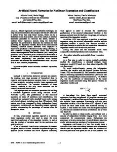
2.5  10^(-6) meters. We have also reduced the number of bands to 200 with 24 water absorption bands being removed. The false color image is visually shown in Figure 1(a). This image contains 10 ground truth classes which can be visually shown in Figure 1(b). In this experiment, we randomly sample 60 pixels of the data in each class as the training samples and the remaining as the test samples, and the detailed information is shown in Table 1. The classification accuracy for each class using different classifiers is also shown in Table 1 and the classification maps are shown in Figure 1(c)-(f). The residual and optimal tolerance parameters for each greedy algorithm mentioned above are default. The optimal parameters for the KNJCRC are   1e  7 , T  81 and K  50 , for the NJCRC are   1e  5 , T  81 and K  55 , where the corresponding optimal neighboring size for JSRC is T  25 . Besides, the parameters for SVM are obtained by 10 fold cross-validation. It is shown from Table 1 that by mapping the original spectral feature into a higher kernel feature space, the proposed algorithm outperforms the other classification algorithms, and is superior to its linear version algorithm. The second hyperspectral image used in this paper is the 115-band ROSIS image Centre of Pavia of size 776  485, for which we use only 102 bands with the 13 water absorption bands removed. The false color image can be visually shown in Figure 2(a). There are 9 classes of interests as shown by the ground truth map in Figure 2(b),  in this experiment, we randomly sample 20 pixels per class of the data as the training samples and the remaining as the test samples, and the detailed is shown in Table 2 which contains the classification accuracy for each class using various and the classification maps are shown in Figure 2(c)-(f). It is observed that we can draw the same conclusion with the first experiment.

classification via column generation technology For the nonlocal joint representation model, we can also extend the S K  B K into the feature space. We first map all the pixels in the spatial window sized T T  K  into the kernel feature space, then calculate the correlation between every kernel signal in the neighborhood window and the test kernel signal sc , and finally sort all kernel signals in the order of descending correlation. We select the first K ones from all the T kernel signals and consider them also share a “common collaborative pattern” in the feature space. The nonlocal kernel joint signal matrix can be represented in the kernel feature space as:

 1, 1  1,  K      SK    A       A  ΨK      N ,1 N , K   

(10)

ΨK

where Ψ K is the kernel collaborative coefficient matrix, and the function (6) can be extended as : ˆ   arg min  K K

 S

K



 A  K

2 F

  K

ˆ Once the coefficient matrix  K classification rule is denoted as:

ˆ class ( sc )  arg min S K    A i   K ,i i 1,, M

2 F



(11)

is obtained, the 2 F

ˆ /  K ,i

2 F

(12)

where   Ai  is a sub-part of   A  in class i , and ˆ  denotes the portion of the recovered kernel  K ,i collaborative coefficients corresponding to the entire training samples in the i th class.

4. CONCLISIONS 3.

EXPERIMENTAL RESULTS AND ANALYSIS

In this paper,  we propose a new HSI classification technique based on collaborative representation in a nonlinear feature space induced by column generation kernel method. The nonlocal contextual correlation is incorporated to constrain the dominated representation through the joint collaboration representation. The kernel technique in this paper is different from the conventional kernel mapping in RKHS feature space by kernel trick.  The column generation directly treats the similar

In this section, we demonstrate the effectiveness of the proposed algorithm on two hyperspectral images. The classical classifier SVMs with RBF kernel [4], JSRC [7] and NJCRC [2] are used as benchmarks in this paper. The first hyperspectral image in this paper was gathered by AVIRIS sensor over the Indian Pines test site in North-western Indiana and consists of pixels and 224 spectral reflectance bands in the wavelength range 0.4–

443

Table T 1. Classificattion accuracy(%) ffor the Indiana Pin ne image on the test t set using differ erent classifiers

measures bettween spectraal pixels as feature, fe while the conventional kernel methood often replaces the origginal feature vectoor as implicitt kernel featu ure by the innner product operration. The extensive e experimental ressults clearly sugggest the prooposed metho od can achiieve competitive cclassification results. Our further f work will focus on  morre brilliant conntextual inform mation extracction which automaatic obtain thee joint signal matrix to furrther improve the cclassification performance. p

Class C 1 2 3 4 5 6 7 8 9 10 OA Kappa K

Train 60 60 60 60 60 60 60 60 60 60

Test 1368 770 423 670 418 912 2395 533 1205 326

600

9020

SVM 0.6923 0.7792 0.9125 0.9418 0.9952 0.7160 0.5908 0.7992 0.9245 0.7178 0.7563 0.7203

JSRC 0.8509 0.9091 0.9409 0.9970 1 0.7971 0.6731 0.8180 0.9593 0.9479 0.8412 0.8177

NJCR RC 0.939 93 0.9416 0.917 73 0.997 70 1 0.974 48 0.777 79 0.968 81 0.974 43 1 0.914 49 0.9018

KNJCRC 0.8882 0.9948 0.9456 0.9910 1 0.9276 0.8342 0.9306 0.9876 0.9969 0.9222 0.9100

5. REFE ERENCES [1] L. Zhang, M M.Yang, X. Feng, Y. Ma, and D.. Zhang,“Collaborrative Representatioon based Classiification for Facce Recognition,”A Arxiv preprint arXi Xiv:1204.2358, 2012. [2] J. Li, H. Zhhang, L. Zhang and Y. Huang., “Hyperspectral Im mage Classificationn by Nonlocal Joint Collaborativee Representation with Locality-adapptive Dictionary,”” IEEE Trans. Geosci. G Remote SSens., submitted [3] J. Bi, T. Z Zhang and K.P. Bennett., B “Colum mn-generation booosting (a)

methods forr mixture of keernels,” in Confeerence on Knowl wledge

(b)

(c)

Discovery iin Data: Proceeedings of the tenth t ACM SIGK GKDD internationall conference on Knowledge K discovvery and data miining, 2004, pp. 5211-526. [4] C.I. Chang, "Hyperspectral im maging: Techniquees for spectral deteection and classificaation", Springer Us, U vol. 1, 2003. [5] X. Yuan, X. Liu, and S. Yann, “Visual Classifiication with Multii-task Joint Sparse R Representation,” IEEE I Trans. Imagee Process., to appeear. [6] H. Zhang, A.C. Berg, M. Maire, and J. Malik, “SVM-K KNN: Discriminativve Nearest Neighhbor Classification n for Visual Cateegory Recognition,”in Proc. IEEE Computer C Society Conf.Computer V Vision (d) (e) (f) Figurre 2.Classification n results of Centtre of Pavia imag ge: (a) false coloor imag ge, (R:102, G:56 ,B B:31), (b) ground ttruth (c) SVM, (d)) JSRC, (e)NJCRC C, (f) KNJCRC K

Recognition, 2006, pp. 2126–2136. and Pattern R [7] Y. Chen, N.. M. Nasrabadi, and T. D. Tran, “Hyperspectral Im mage Classificationn Using Dictionarry-Based Sparse Representation,” IIEEE Trans. Geosci. Remote Sens., vol. 49, no. 10,, pp. 3973–3985, Oct.

Taable 2. Classificatio on accuracy(%) foor the Centre of Paavia image on the test t set using diffeerent classifiers JSRC NJC Cllass Train Test T SVM CRC KNJCRC 1 20 5290 5 0.9809 1 1 1 2 20 3486 3 0.8448 0.8890 0.93 317 0.8964 3 20 958 9 0.9614 0.9676 0.89 904 0.9259 4 20 2120 2 0.8542 0.9443 0.51 170 0.9920 5 20 1069 0.8877 0.9476 1 0.9355 6 20 4869 4 0.8316 0.7989 0.98 881 0.9499 7 20 7267 7 0.8563 0.9180 0.96 622 0.9040 8 20 3102 3 0.9700 0.9923 1 0.9997 9 20 1599 0.9950 0.9287 0.74 448 0.7967 OA O 0.8967 0.9225 0.92 292 0.9400 180 29 9940 Kaappa 0.8793 0.9092 0.91 162 0.9295

2011.

(a)

(b)

(c)

6. ACKNOWLE A EDGEMENTS S Thiss work was supported s in ppart by the National N Basicc Reseearch Program m of China ((973 Program)) under Grantt 2011CB707105, by y the National N Natural Sciencee Foundation off

(d) (e) (f) Figure 1.Classificcation results of Inndian Pines imagee: (a) false color iimage (R:57 G:27 B:177) (b) ground trutth (c) SVM, (d) JSRC, (e) NJCR RC, (f) KNJCRC

Chin na under Grants 612013442 and 40930 0532 and byy LIESMARS Speciaal Research Funnding. 

444