A Note on efficient computation of Haplotypes via Perfect Phylogeny Vineet Bafna∗
Dan Gusfield†
Sridhar Hannenhalli‡
Shibu Yooseph§
September 5, 2003
1
Introduction
With the completion of the draft sequencing of the human genome [13, 18], a natural next step is to identify, and characterize, the variations that explain the diversity of the human species. Much of the variation can be explained by Single Nucleotide Polymorphisms (SNPs) which correspond to point mutations that have accumulated in the population. Large scale resequencing and genotyping efforts are underway that aim to construct a map of SNPs in the human genome. It is expected that such a map will be invaluable in identifying genetic causes of complex disorders. Humans, being diploid, contain two copies of every chromosome (and therefore every SNP), inherited from the mother, and father. Most current strategies for SNP determination allow the demarcation of markers as being homozygous or heterozygous (i.e. whether the maternal and paternal alleles are identical or not), but not haplotyping, i.e., determining which alleles are maternal, and which are paternal. Obtaining haplotypes have been shown to increase the power of mapping of disease genes. In the absence of biological techniques, various statistical [7, 17, 15], and combinatorial algorithms [1, 4, 6, 11] have been devised to extract haplotype information from genotype data. This is of partiular interest in regions where there is little, or no recombination, and the various ∗ Computer † Dept.
Science Department, UC San Diego, Email:
[email protected] of Computer Science, 3051 Engineering II, University of California, One Shields Avenue, Davis, CA 95616.
Email:
[email protected] Research Supported by NSF grant DBI-9723346 and EIA-0220154 ‡ § Informatics
Research,
Applied
Biosystems,
45
W.
[email protected]
1
Gude
Drive,
Rockville,
MD
20850.
Email:
SNPs are tightly linked. Indeed, initial studies [5] point to varying recombination rates across the genome, and reveal many regions with little or no genetic recombination in the population. Motivated by these considerations, Gusfield [11] formulated a combinatorial version of the haplotyping problem. Given a region in which there have been 0 recombination events, and making the infinite sites assumption (each mutation hits a new site on the genome), the set of haplotype sequences form a perfect phylogeny. The PPH problem, as formulated in [11] is stated as follows: Given n diploid sequences, can they be resolved into a set of 2n haploid sequences which form a perfect phylogeny. If they can, find an implicit representation of all the solutions, so that each solution can be explicitly generated in O(m) time. Gusfield [11] presented an efficient algorithm that solved the PPH problem in O(nmα(nm)) time. However, the proof made use of established, difficult results in the matroid and graph theory literature, which are difficult to implement, and a more direct approach to solving the problem was desired. Subsequent work [1, 6] closed this gap, showing direct, easy to understand, yet efficent solutions. Both solutions have complexity Θ(nm2 ) which is higher than the O(nmα(nm)) solution. Another implementation [3, 2] follows the high-level idea in [11], but runs in O(nm2 ) time. The algorithm in Bafna et al. [1] has four steps:genotype graph construction, Edge assignment, haplotype matrix creation, and validation. Each step, except for the first could be accomplished in time O(nm + m2 ), and the Θ(nm2 ) bound is essentially for the first step of genotype graph construction, so any reduction in the time for the first step reduces the overal running time. Reducing that time was left as an open problem in [1]. The algorithm in Eskin et al. [6] also has a first step which is very similar to the first step in [1], also taking Θ(nm2 ) time. The time-bound established for the steps needed beyond the first step is O(nm2 ). Additionally, if there is more than one solution to the PPH problem, there is a space efficient representation for all of the possible solutions, as well as a time efficient algorithm for exposing all solutions ([1, 6]). However, the number of PPH solutions may be very large, and it is an open problem to select one that is optimal under some reasonable criterion. In this short note, we address the issue of whether the first steps of the algorithms in [1, 6] can be sped-up to O(nm + m2 ) time, which would imply an O(nm) time-bound for the PPH problem. In addition, if there are multiple solutions, we address the question of finding one that is optimal w.r.t the number of haplotypes.
2
We were motivated to try to improve the running time of the first step by three facts: First, the the output of the first step is of size O(m2 ); second the result in [11] shows that o(nm2 ) time is possible for the PPH problem; third, the fact established in the Section 3 shows that if the PPH problem could be solved in O(nm + m2 ) time, then it can be solved in O(nm) time. For the second problem, minimizing the number of possible haplotypes is reasonable based on the considerations of parsimony. Indeed, many haplotyping algorithms use the parsimony criterion implicitly, or explicitly. We give reductions that suggests that the answer to both questions is “no”. For the first problem, we show that computing the output of the first step (in either method) is equivalent to Boolean matrix multiplication. Therefore, the best bound we can presently achieve is O(nmω−1 ), where ω ≤ 2.52 is the exponent of matrix multiplication. Thus, any linear time solution to the PPH problem, likely requires a different approach. For the second problem of computing a PPH solution that minimizes the number of distinct haplotypes, we show that the problem is NP-hard using a reduction from Vertex Cover [8].
2
The PPH solution in [1]
A matrix-oriented approach is taken in [1] to solve the PPH problem. In our discussion we will use the same notations as in that work. The input to the problem is a n × m genotype matrix M with M [i, j] ∈ {0, 1, 2}. The i-th row M [i, ∗] describes the genotype of species si , and each location j where M [i, j] = 2 is a polymorphic site. Each column cj = M [∗, j] is a polymorphic locus. The goal is to generate a 2n × m haplotype-matrix M 0 , with M 0 [i, j] ∈ {0, 1}. A 2n × m haplotype-matrix M 0 is an expansion of a n × m genotype matrix M , if the following hold. 1. Each row M [i, ∗] expands to two rows denoted by M 0 [i, ∗], and M 0 [i0 , ∗]. 2. For all j s.t. M [i, j] ∈ {0, 1}, M [i, j] = M 0 [i, j] = M 0 [i0 , j]. 3. For all j s.t. M [i, j] = 2, M 0 [i, j] 6= M 0 [i0 , j]. Also, as discussed in the previous section, the set of haplotypes must form a perfect phylogeny. We use the no-four-gamtes characterization of perfect phylogeny, which has been independently established many times (for an exposition see [9, 10]). Define a complete-pair-matrix as matrix with 2 columns, containing each of the rows in {00, 01, 10, 11}. The classical theorem is that a 2n × m
3
binary matrix M 0 defines a unrooted perfect phylogeny if and only if no submatrix M 0 [∗, (j1 , j2 )] formed by selecting the two columns j1 , j2 , is a complete-pair-matrix. Columns j, k in a genotype matrix M are companions, if there exists a row i such that M [i, j] = M [i, k] = 2. Row i is said to be a companion row for columns j and k. Companion columns j, k are said to be forced in-phase if the expansion of the non-companion rows contains {00, 11}; similarly, companion columns j, k are said to be forced out-of-phase if the expansion of the non-companion rows contains {01, 10}. The forcing relations between companion columns are described using an indicator function E. For companion columns j, k, E(j, k) = 0 if these columns are forced in-phase and E(j, k) = 1 if they are forced out-of-phase. The task is to determine the value of E(j, k) for those companion columns j, k that are not forced, i.e., for which the expansion of non-companion rows does not contain either {00, 11} or {10, 01}. In [1] it is shown that a solution to the PPH instance exists iff the indicator function setting of companion column pairs satisfies certain properties. The algorithm proposed in [1] to solve the PPH problem has four main steps: 1. Genotype graph construction: In this step the genotype graph GM = (J, Ef ∪ En ) is constructed from the genotype matrix M and the indicator function E is set appropriately for each edge in Ef (see below). 2. Assignment: The indicator function E is set appropriately for each edge in En . 3. Haplotype matrix creation: The haplotype matrix M 0 is produced from the genotype matrix M using the indicator function assignments to the edges in GM . 4. Validation: M 0 is checked to see if it admits a perfect phylogeny. The genotype graph GM = (J, Ef ∪ En ) is constructed from the genotype matrix M as follows: J is the set of columns in M . An edge (j, k) ∈ Ef iff j and k are either forced in-phase or out-of-phase. Also, E(j, k) = 0 iff they are forced in-phase and E(j, k) = 1 iff j they are forced out-of-phase. Finally, an edge (j, k) ∈ En iff j and k are companion columns but are not forced to be in-phase or out-of-phase. The graph construction phase takes O(nm2 ) using the obvious algorithm. The indicator function assignment step operates on GM . This involves a DFS-like traversal on the edges in Ef and uses the properties of GM to assign the indicator function to edges in En . This
4
step takes O(|J|+|Ef ∪En |) = O(m2 ). The last two steps of the algorithm can both be accomplished in O(nm) time. Thus, the bottleneck to obtaining a faster algorithm for the PPH problem is the graph construction step. In Section 4 we show that constructing GM is equivalent to boolean matrix multiplication problem.
3
O(nm + m2 )-time implies O(nm)-time
Theorem 1: If the PPH problem can be solved in O(nm + m2 ) time, by any method, then it can be solved in O(nm) time. Proof:
This is certainly true if m = O(n), since O(nm + m2 ) = O(nm) in that case. So assume
that m = Ω(n). The genotype matrix M is n by m, so a perfect phylogeny P that solves the PPH problem for input M which will have 2n leaves. Every internal node of P must have at least two children, so P can have at most 2n − 1 internal nodes, and hence at most 4n − 1 nodes and 4n − 2 edges overall. Each mutation is assigned to only one edge in P , so for any genotype matrix M where m > 4n − 2, either there is no PPH solution for M , or there must be duplicate columns in M , and at most 4n − 2 distinct columns. Using radix sort (considering each column as a binary number), duplicate columns can be grouped together in O(nm) time. If we want only a single PPH solution, we can remove all but one copy of each duplicate column, leaving at most 4n − 2 distinct columns. This leaves a PPH problem with an input matrix M 00 of size n by m00 , where m00 = O(n), which can be solved in O(n2 ) = O(nm) time. Hence, the overall time bound to find one PPH solution, including the time for the radix sort is O(nm). If we want to find a representation of all the solutions, then we can proceed in one of two ways. It was stated in [11] that once one solution to the PPH problem is found (by whatever method), an implicit representation of all the solutions can be found in O(m) additional time. However, that approach is complex, and has not been implemented. A simpler approach that is more easilly implemented is shown next.
5
Even if there are k > 2 copies of a given column v in M , in any PPH solution there are at most two distinct ways that those k columns will be expanded in a solution M 0 . This follows from the fact that each pair v, w of the k columns is a companion pair and the columns are identical, so knowing how v is expanded and knowing the value of E(v, w), completely determines the expansion of w. So assume we remove all but two copies v, w of a column that has k > 2 copies in M . Let M denote the reduced matrix. A PPH solution for M where E(v, w) = 0 is interpreted as a PPH solution where all of the k columns are expanded the same way (in-phase). However, a PPH solution where E(v, w) = 1 expands columns v and w differently (out-of-phase). That solution actually corresponds to 2k − 2 solutions, where we choose arbitrarilly which of the two expanions to use for any of the k columns other than v and w. So even when k > 2, we can again use O(nm)-time to reduce the input to a problem of size n by m00 , where m00 = O(n), and so we can find an implicit representation of all the PPH solutions in O(nm) time, if the PPH problem can be solved in O(nm + m2 ) time.
4
♣
Equivalence of genotype graph construction and boolean matrix multiplication
Definition: Given an n × m matrix P in which the entries are drawn from the alphabet Σ, we will use Pab to denote the template matrix derived from P for the template ab (where a, b ∈ Σ) as follows: Pab is an m × m boolean matrix in which an entry Pab [j, k] = 1 iff P [i, j] = a and P [i, k] = b, for some 1 ≤ i ≤ n. Lemma 2:
The genotype graph GM = (J, Ef ∪ En ) can be constructed by querying template
matrices M00 , M01 , M10 , M11 , M20 , M02 , M21 , M12 , and M22 . Proof:
An edge (j, k) ∈ Ef ∪En iff M22 [j, k] = 1. Edge (j, k) ∈ Ef and E(j, k) = 0 iff (M22 [j, k] =
1 and (M00 [j, k] = 1 or M20 [j, k] = 1 or M02 [j, k] = 1) and (M11 [j, k] = 1 or M21 [j, k] = 1 or M12 [j, k] = 1)). Similarly, (j, k) ∈ Ef and E(j, k) = 1 iff (M22 [j, k] = 1 and (M10 [j, k] = 1 or M20 [j, k] = 1) and (M01 [j, k] = 1 or M02 [j, k] = 1)). We assume that an edge (j, k) ∈ Ef cannot have both E(j, k) = 0 and E(j, k) = 1, as this implies that M does not have a PPH solution [1].
6
Finally, edge (j, k) ∈ En iff (j, k) ∈ Ef ∪ En and (j, k) ∈ / Ef .
♣
Lemma 3: Denote by T (h, k, l), the time to multiply two boolean matrices of diemensions h × k, and k × l respectively. Given an n × m matrix M , a template matrix Mab can be computed in time O(T (m, n, m). Proof:
Define boolean matrices Xm×n and Yn×m as follows. Entry X[j, i] = 1 iff M [i, j] = a,
where 1 ≤ i ≤ n and 1 ≤ j ≤ m. Entry Y [i, j] = 1 iff M [i, j] = b, where 1 ≤ i ≤ n and 1 ≤ j ≤ m. Let Z = X.Y . We claim that Mab = Z. To see why, note that entry Z[j, k] =
n X
X[j, i].Y [i, k],
where 1 ≤ i ≤ n and 1 ≤ j ≤ k ≤ m
i=1
Thus Z[j, k] = 1
iff
X[j, i] = 1 and Y [i, k] = 1, for some 1 ≤ i ≤ n
iff
M [i, j] = a and M [i, k] = b
iff
Mab [j, k] = 1 ♣
Corollary 4:
GM = (J, Ef ∪ En ) can be constructed in O(nmω−1 ), where ω is the constant in
boolean matrix multiplication. Proof:
Consider the boolean matrices Xm×n and Yn×m defined in Lemma 3. Since m ≤ n, we
can partition them as shown
X = [X(1) X(2) .. X(n/m)] and Y =
Y (1) Y (2) .. Y (n/m)
where each X(i) is an m × m matrix and each Y (j) is also an m × m matrix. Thus
n/m
X.Y =
X
X(i).Y (i)
i=1
Let T (m) denote the time taken to multiply two m × m boolean matrices. Thus, the total time n )T (m)). Since T (m) = O(mω ), it follows that the total time taken taken to compute X.Y is O(( m
is O(nmω−1 ).
♣ 7
Lemma 5:
Let TG (n, m) be the time to construct a genotype graph, given an n × m genotype
matrix M . two boolean matrices with dimensions m1 × n, and n × m2 respectively can be multiplied in time O(TG (n, m1 + m2 ). Proof:
Consider two boolean matrices Xm1 ×n and Yn×m2 . Let Am1 ×n be a matrix derived from
X by replacing each 1 by a 2. Similarly, let Bn×m2 be a matrix derived from Y by replacing each 1 by a 2. We define the genotype matrix Mn×(m1 +m2 ) = [AT B], where AT denotes the transpose of A. Note that the j th column of B appears as the (m1 + j)th column in M . Let GM = (J, Ef ∪ En ) denote the genotype graph for M and let Zm1 ×m2 = X.Y . We claim that Z[j, k] = 1 iff (j, m1 + k) ∈ Ef ∪ En . The proof follows.
Z[j, k] = 1
iff
X[j, i] = 1 and Y [i, k] = 1, for some 1 ≤ i ≤ n
iff
A[j, i] = 2 and B[i, k] = 2
iff
M [i, j] = 2 and M [i, m1 + k] = 2
iff
(j, m1 + k) ∈ Ef ∪ En
For genotype matrix Ma×b , let T (a, b) denote the time taken to construct the genotype graph GM . From the above reduction, it follows that the time taken to compute the product of Xm1 ×n and Yn×m2 is O(T (n, m1 + m2 )). ♣
5
Complexity of MIN-PPH problem
When the solution to the PPH problem is not unique, we seek a criteria to identify a solution that is more biologically compelling than the others. One criteria that has strong empirical and theoretical support is that of maximum parsimony, i.e., a solution that uses the fewest number of distinct haplotypes to explain the given genotypes. The parsimony criteria is discussed in [14, 12, 16, 19] in the context of the haplotyping problem, where a set of haplotypes must explain the genotypes but are not required to solve the PPH problem. In particular, in [12, 16] the parsimony criteria was shown to be effective in identifying highly accurate haplotyping solutions (in simulations and in the few cases where we know the true underlying haplotypes). A natural conjecture is that this is also 8
true in the context of the PPH problem. Hence, if there is more than one PPH solution, it is of interest to obtain and examine a most-parsimonious PPH solution, if only to test (in cases when we know the true underlying haplotypes) the conjecture that a most-parsimonious PPH solution is most often highly accurate. Unfortunately, obtaining a most-parsimonious PPH solution is likely to be much more difficult than finding an arbitrary PPH solution, as we show next. The MIN-PPH problem: Input: An instance of the PPH problem, and an integer d. Output: Does a PPH solution exist with d or fewer distinct haplotypes? Theorem 6: MIN-PPH is NP-Complete. Proof:
The problem is clearly in the class NP. To show that it is NP-Hard, we show a reduction
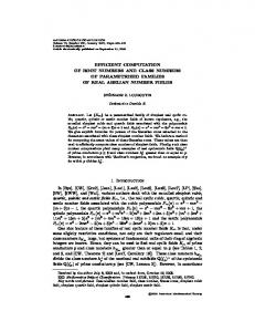
from the Vertex Cover Problem [8]. Let graph G = (V, E) be the input to the Vertex Cover Problem. We will construct a genotype set G with |V | + |E| genotypes and 2|V | + |E| sites, as the corresponding instance of the MIN-PPH problem. We define G = {a1 , a2 , . . . , a|V | } ∪ {b1 , b2 , . . . , b|E| }, where genotype ai is associated with vertex vi and genotype bj is associated with edge ej = (vi1 , vi2 ). We now define the settings at each site for each genotype. Genotype ai , where 1 ≤ i ≤ |V |, has a 1 at sites i and |V | + i, and a 0 at each of the remaining sites. Genotype bj , where 1 ≤ j ≤ |E|, has a 2 at sites i1 ,i2 , and 2|V | + j, and a 0 at each of the remaining sites. Figure 1 shows an example of the reduction. In this example, the genotype set G has eight genotypes - the four ai ’s are associated with V and the four bj ’s are associated with E. Each genotype has 2|V | + |E| = 12 sites. Vertex cover of {v1 , v3 } for graph G corresponds to PPH solution H with 10 distinct haplotypes for G, where H = {100010000000,010001000000, 001000100000,000100010000, 010000001000,100000000100,010000000010,000100000001,100000000000,001000000000}.
The last
two haplotypes in H correspond to vertices v1 and v3 respectively. We make two observations about the nature of any solution for the MIN-PPH instance G • (Observation 1) Each genotype ai is homozygous in every site, i.e. each ai is also a haplotype. Note that this haplotype is unique to ai ; that is, it cannot be used to resolve any other genotype in G. The reason for this is due to the 1 at site |V | + i. 9
v1
e1
v2
a1 = 100010000000 a2 = 010001000000 a3 = 001000100000 a4 = 000100010000 b1 = 220000002000 b2 = 202000000200 b3 = 022000000020 b4 = 002200000002
e3
e2 v3 e4
v4 G = (V, E)
G = {a1 , a2 , a3 , a4 , b1 , b2 , b3 , b4 } Figure 1: An example showing the reduction. • (Observation 2) For each genotype bj , one of the two haplotypes that resolve it, namely the one that has a 1 at site 2|V | + j, is unique to bj . We claim that the graph G has a vertex cover of size k iff the MIN-PPH instance has a solution with d = |V | + |E| + k distinct haplotypes. The proof follows. (→) Suppose that G has a vertex cover of size k. We will construct a set of haplotypes H as follows. From observation 1, it follows that the ai ’s will contribute |V | distinct haplotypes to H. Now, consider the genotype bj that is associated with edge ej = (vi1 , vi2 ). W.l.o.g., assume that vi1 is a vertex that is part of the vertex cover. Then bj will be resolved into two haplotypes as follows. The first haplotype (denote it as a VC-haplotype) has a 1 at site i1 and a 0 at each of the remaining sites, and the second haplotype has a 1 at sites i2 and 2|V | + j, and a 0 at each of the remaining sites. From observation 2, the second haplotype is unique to bj . Furthermore, since the vertex cover has size k, there will be k distinct VC-haplotypes. Thus, H has |V | + |E| + k distinct haplotypes. By construction, each genotype in G is resolved by haplotypes from H. We now show that H is a PPH solution. Let’s consider the haplotypes which have two 1’s. There is one for each ai genotype and one for each bj genotype. In the case of ai , the second 1 is in column |V | + i ≤ 2|V |, which has only 0’s in the other a-derived haplotypes (because, the only a-derived haplotype with a 1 in column |V | + i is an ai -derived haplotype), and all the b-derived haplotypes also have a 0 in column |V | + i (because every entry in a b-derived haplotype is 0 in columns |V | + 1 through 2|V |). Hence a pair of columns which are 1,1 in an a-derived haplotype, cannot be 0,1 in
10
any of the other haplotypes. Now consider the bj -derived haplotype that has two 1’s. Its second 1 is in column 2|V | + j. Every a-derived haplotype has a 0 entry in that column, and among the b-derived haplotypes, only one bj -derived haplotype has a 1 in that column. Hence a pair of columns which are 1,1 in an b-derived haplotype, cannot be 0,1 in any of the other haplotypes. It follows that H contains no complete-pair submatrix, and so is a PPH solution. (←) Suppose that G has a PPH solution H containing |V | + |E| + k distinct haplotypes. We will show how to construct a vertex cover of size k in G. First, consider the genotype ai . From observation 1, each ai contributes a distinct haplotype in H. Next, consider the genotype bj that is associated with edge ej = (vi1 , vi2 ). From observation 2, we have that bj contributes one distinct haplotype to H. The second haplotype (denote it by hj ) contributed by bj may or may not be unique. Furthermore, this second haplotype has a 1 in exactly one of site i1 or i2 , and a 0 at each of the remaining sites. This is because for H to be a PPH solution, the sites (columns) i1 and i2 have to be forced out-of-phase because genotype ai1 has a 1 at site i1 and 0 at site i2 while genotype ai2 has a 0 at site i1 and a 1 at site i2 . Let H 0 denote the set of hj ’s. From the preceeding arguments, |H 0 | = k. Define the vertex set V 0 = {vi |∃hj ∈ H 0 that has a 1 at site i}. For each 1 ≤ j ≤ |E|, genotype bj (which is associated with edge ej ) has some h ∈ H 0 that resolves this genotype; it follows that V 0 is a vertex cover of size k for the graph G. ♣
References [1] V. Bafna, D. Gusfield, G. Lancia, and S. Yooseph. Haplotyping as perfect phylogeny: A direct approach. Technical report, U.C. Davis, 2002. To appear in Jnl. Computational Biology. [2] R.H. Chung and D. Gusfield. Empirical exploration of perfect phylogeny haplotyping and haplotypers. In Proceedings of the 9’th International Conference on Computing and Combinatorics, volume 2697 of LNCS, pages 5–19, 2003. [3] R.H. Chung and D. Gusfield. Perfect phylogeny haplotyper: Haplotype inferral using a tree model. Bioinformatics, 19(6):780–781, 2003. [4] Andrew Clark. Inference of haplotypes from PCR-amplified samples of diploid populations. Mol. Biol. Evol, 7:111–122, 1990. 11
[5] M. Daly, J. Rioux, S. Schaffner, T. Hudson, and E. Lander. High-resolution haplotype structure in the human genome. Nature, 29:229–232, 2001. [6] E. Eskin, E. Halperin, and R.M. Karp. Large scale reconstruction of haplotypes from genotype data. In Proceedings of Seventh Annual International Conference on research in Computational Molecular Biology (RECOMB), pages 104–113, 2003. [7] L. Excoffier and M. Slatkin. Maximum-liklihood estimation of molecular haplotype frequencies in a diploid population. Mol. Bio. Evolution, 12:921–927, 1995. [8] M. Garey and D. Johnson. Computers and intractability. Freeman, San Francisco, 1979. [9] D. Gusfield. Efficient algorithms for inferring evolutionary history. Networks, 21:19–28, 1991. [10] D. Gusfield. Algorithms on Strings, Trees and Sequences: Computer Science and Computational Biology. Cambridge University Press, 1997. [11] D. Gusfield. Haplotyping as Perfect Phylogeny: Conceptual Framework and Efficient Solutions (Extended Abstract). In Proceedings of RECOMB 2002: The Sixth Annual International Conference on Computational Biology, pages 166–175, 2002. [12] D. Gusfield.
Haplotype inference by pure parsimony.
In R. Baeza-Yates, E. Chavez,
and M. Chrochemore, editors, 14’th Annual Symposium on Combinatorial Pattern Matching (CPM’03), volume 2676 of Springer LNCS, pages 144–155, 2003. [13] International Human Genome Sequencing Consortium. Initial sequencing and analysis of the human genome. Nature, 409:860–921, 2001. [14] G. Lancia, C. Pinotti, and R. Rizzi. Haplotyping populations: Complexity and approximations, technical report dit-02-082. Technical report, University of Trento, 2002. [15] T. Niu, Z. Qin, X. Xu, and J.S. Liu. Bayesian haplotype inference for multiple linked singlenucleotide polymorphisms. Am. J. Hum. Genet, 70:157–169, 2002. [16] S. Orzack, D. Gusfield, , J. Olson, S. Nesbitt, and V. Stanton. Analysis and exploration of the use of rule-based algorithms and consensus methods for the inferral of haplotypes. Genetics, to appear.
12
[17] M. Stephens, N. Smith, and P. Donnelly. A new statistical method for haplotype reconstruction from population data. Am. J. Human Genetics, 68:978–989, 2001. [18] J.C. Venter, M.D. Adams, G.G. Sutton, A.R. Kerlavage, H.O. Smith, and M. Hunkapillar. Shotgun sequencing of the human genome. Science, 280:1540–1542, 1998. [19] L. Wang and Y. Xu. Haplotype inference by maximum parsimony. Bioinformatics, to appear.
13