A Note on Least Squares Support Vector Machines - Semantic Scholar

A Note on Least Squares Support Vector Machines

Wei Chu

[email protected]

Chong Jin Ong

[email protected] [email protected]

S. Sathiya Keerthi

Control Division, Department of Mechanical Engineering, National University of Singapore, 10 Kent Ridge Crescent, Singapore, 119260

Abstract In this paper, we propose some improvements for the implementations of least squares support vector machine classifiers (LS-SVM). An improved conjugate gradient scheme is proposed for solving the optimization problems in LS-SVM, and an improved SMO algorithm is put forward for the general unconstrained quadratic programming problems which is the case of LS-SVM without the bias term. Numerical experiments are carried out to verify the usefulness of these improvements. We also attempt to point out the potential weaknesses in Bayesian framework for LS-SVM classifiers proposed by Van Gestel et al. (2002).

1. Introduction Least squares support vector machine classifiers (LS-SVM) have been proposed by Suykens and Vandewalle (1999) as an interesting reformulation of the standard support vector machines (SVM) (Vapnik, 1995). LS-SVMs are closely related to the kernel version of ridge regression (Saunders et al., 1998) and Gaussian processes (Williams and Rasmussen, 1996), but additionally emphasize the primal-dual formulation from optimization theory. A careful empirical study by Van Gestel et al. (2000) has shown that LS-SVMs is comparable to standard SVM in terms of generalization performance. The nature links between LS-SVM classifiers and kernel Fisher discriminant analysis have been established by Van Gestel et al. (2002). The formulation has been further extended towards kernel principal component analysis (Suykens et al., 2002). As for the algorithm designs, Suykens et al. (1999) employed the conjugate-gradient methods to solve the KKT system of linear equations, in which the solution to two linear systems with the order of the number of training samples are required. The well-known SMO algorithm for SVM has been extended to LS-SVMs by Keerthi and Shevade (2003). Cross validation is usually used for model selection, while a Bayesian approach has been proposed by Van Gestel et al. (2002) to provide an alternative for hyperparameter tuning. In this paper, we propose some improvements for the existent algorithms for LS-SVMs: for the conjugate-gradient algorithm design, we give a more efficient scheme in which only one linear system need to solve; for the cases without the bias term, i.e. unconstrained quadratic programming problems, we give an improved SMO algorithm; as for model selection, we attempt 1

to point out the potential weaknesses in the Bayesian framework for LS-SVMs proposed by Van Gestel et al. (2002). The paper is organized as follows: we review the LS-SVM formulation in section 2, and then propose the improved scheme for conjugate gradient algorithm to solve the consequent optimization problem in section 3; we put forward an improved SMO algorithm for the general unconstrained quadratic programming problems in section 4; we carry out numerical experiments on some benchmark data sets with different sizes to verify our improved schemes in section 5; we give some comments on the Bayesian design for LS-SVM proposed by Van Gestel et al. (2002) in section 6, and conclude in section 7. 2. LS-SVM Formulation Suppose that we are given a training data set of n data points {xi , yi }ni=1 , where xi ∈ Rd is the i-th input vector and yi ∈ R is the corresponding i-th target. For binary classification problems yi takes only two possible values {−1, +1}, while for regression yi takes any real value. In kernel designs, we employ the idea to transform the input patterns into the reproducing kernel Hilbert space (RKHS) by a set of mapping functions φ(x). Let us denote the reproducing kernel in RKHS as K(x, x′ ), which is defined as K(x, x′ ) = φ(x) · φ(x′ )

(1)

In the RKHS, a linear classification/regression is performed. The discriminant function takes the form n X y(x) = w · φ(x) + b (2) i=1

where w is the weight vector in RKHS, and b ∈ R which is called as the bias term.1 The discriminant function of LS-SVM classifiers (Suykens and Vandewalle, 1999) is constructed by minimizing the following primal problem: n 1 CX 2 min P (w, b, ξ) = kwk2 + ξ (3) w,b,ξ 2 2 i=1 i subject to the equality constraints yi − (w · φ(xi ) + b) = ξi ∀i, where the regularization parameter C > 0. Note that the formulation for classifier design is same as that for regression. Traditionally an inequality constraint is exploited on the slack variables ξi to punish the misclassified patterns only. Nevertheless, the formulation of LS-SVM produces penalty to all the patterns if their discriminant function does not equal to the corresponding target value, as the traditional regression formulation does. Standard Lagrangian techniques (Fletcher, 1987) are used to derive the dual problem. The Lagrangian for the primal problem (3) is: n n 1 CX 2 X 2 L(w, b, ξ; α) = kwk + ξ + αi {yi − (w · φ(xi ) + b) − ξi } (4) 2 2 i=1 i i=1 where αi are Lagrangian multipliers, which can be either positive or negative due to the equality constraints. The KKT conditions for the primal problem (3) are: n X ∂L =0⇒w= αi φ(xi ) (5) ∂w i=1 1

The bias term b could be dropped off in the discriminant function, which leads to a simpler problem.

2

n

X ∂L =0⇒ αi = 0 ∂b i=1 ∂L = 0 ⇒ αi = Cξi ∂ξi

(6) ∀i

(7)

Together with the KKT conditions for Lagrangian multipliers {αi }, Suykens and Vandewalle (1999) write them as a linear system, and suggest to solve two linear systems and then combine the results to get the final solution to the KKT linear system. Both the two linear system we solved using conjugate gradient methods are of the order of the number of training samples n. Here we point out that this is not the efficient way for the solution. Actually, the final solution can be obtained by solving one linear system of the order n − 1 only. 3. Conjugate Gradient Design We resort to the dual problem for the solution instead of the KKT linear system. Substituting the KKT conditions (5)∼(7) into the Lagrangian (4) and using the property of reproducing kernel (1), the dual problem of LS-SVM can be finally simplified as n

n

n

X 1 XX max D(α) = − αi αj Q(xi , xj ) + yi αi α 2 i=1 j=1 i=1 s.t. as

Pn

i=1

(8)

αi = 0, where Q(xi , xj ) = K(xi , xj ) + C1 δij . We can write the dual (8) in vector form 1 max D(α) = − αT Qα + αT y α 2

(9)

Pn

αi = 0, where Qij = K(xi , xj ) + C1 δij , y = [y1 , y2 , . . . , yn ]T and α = [α1 , α2 , . . . , αn ]T . · ¸ ¯ Q qn ¯ = Let us define Q = , where q n = [K(x1 , xn ), K(x2 , xn ), . . . , K(xn−1 , xn )]T , y q Tn Qnn ¯ = [α1 , α2 , . . . , αn−1 ]T , and e = [1, 1, . . . , 1]T ∈ Rn−1 . The dual (9) now [y1 , y2 , . . . , yn−1 ]T , α becomes s.t.

i=1

1 T¯ 1 T 1 1 ¯ =− α ¯ Qα ¯− α ¯ q n αn − αn q Tn α ¯ − αn Qnn αn + α ¯ + αn yn ¯Ty max D(α) α ¯ 2 2 2 2

(10)

¯ which comes from the equality constraint in the dual (8). Using the equality where αn = −eT α constraint, the dual problem can be simplified as 1 T˜ ¯ =− α ˜ ¯ Qα ¯ +α ¯Ty max D(α) α ¯ 2

(11)

˜ =Q ¯ − q n eT − eq T + Qnn eeT and y ˜ ij = K(xi , xj ) − K(xi , xn ) − ˜ =y ¯ − yn e, i.e. Q where Q n ˜ i = yi − yn with 1 ≤ i, j ≤ n − 1. K(xj , xn ) + K(xn , xn ) and y ˜ is positive definite provided that Q is positive definite, and then Note that it is easy to show Q T ¯ is valid due to the distinct {αi }. To obtain the solution to the the replacement αn = −e α dual (8), now we can use the standard conjugate gradient algorithm (Fletcher, 1987) for solving ˜α ¯ =y ˜ . Clearly, in the comparison with the scheme proposed by the new n − 1 linear system Q Suykens and Vandewalle (1999), our scheme can save at least 50% computational cost. 3

4. Without the Bias It is also usual to consider the primal problem (3) without the bias term b, such as in P kernel ridge regression (Saunders et al., 1998). When b is dropped off,2 the equality constraint ni=1 αi = 0 vanishes from the dual problem (8). Now the dual problem (8) becomes 1 max D(α) = − αT Qα + αT y α 2

(12)

where Qij = K(xi , xj ) + C1 δij , y = [y1 , y2 , . . . , yn ]T and α = [α1 , α2 , . . . , αn ]T . This is a general quadratic programming problem without any constraints, in which conjugate gradient algorithm can be used directly for solving Qα = y. As for the SMO algorithm design, it is usual to modify one αi at a time instead of updating a pair (Keerthi and Shevade, 2003) since the absence of the equality constraint. Here we put forward a faster scheme in which we keep updating a pair. It is necessary to write down the optimality conditions for the dual (12). The KKT conditions for the dual problem are Fi = 0 ∀i (13) Pn where Fi = yi − j=1 αj Q(xi , xj ). Let us define bup = min Fi and iup = arg min Fi i

i

blow = max Fi and ilow = arg max Fi . i

i

The optimality conditions will hold at a given α iff bup ≥ −τ and blow ≤ τ

(14)

where the tolerance parameter τ > 0, usually 10−3 . Let us now give more details of the improved scheme. Every time we choose the pair (αiup , αilow ) for updating, while keeping others intact. The objective function can be expressed as a Taylor expansion at the old α as follows: ¸ · up ¸T · · ¸T · ¸· ¸ 1 α α ˆ iup − αiup b ˆ iup − αiup Qiup iup Qiup ilow α ˆ iup − αiup − D(ˆ α) = D(α)+ low α ˆ ilow − αilow b ˆ ilow − αilow Qilow iup Qilow ilow α ˆ ilow − αilow 2 α We could simply choose the Newton-Raphson formulation to update the pair. Hence · ¸ · ¸ · ¸−1 · up ¸ α ˆ iup αiup Qiup iup Qiup ilow b = + α ˆ ilow αilow Qilow iup Qilow ilow blow

(15)

Clearly, the increment on D(α) at each updating step is3 ¸T · · ¸−1 · up ¸ 1 bup Qiup iup Qiup ilow b ∆D(α) = low low b Q Q b low up low low 2 i i i i After that, we shall update Fi ∀i,4 and then vote the new bup and blow . Repeat the pair’s updating (15) till the optimality conditions (14) are satisfied. Other optimality conditions could 2

A constant term is usually added in kernel function K(xi , xj ) if the bias is absent. The increment is usually greater than that in the scheme of updating one αi , that might lead to faster convergence. 4 We usually cache all Fi and the diagonal entries of Q in memory for efficiency. 3

4

also be used here, such as the duality gaps (Smola and Sch¨olkopf, 1998; Keerthi and Shevade, 2003). P Note that the dual problem (8) without the constraint ni=1 αi = 0 is equivalent to the maximum a posteriori (MAP) estimate in Gaussian processes for regression (Williams and Rasmussen, 1996) given the covariance function K(xi , xj ) and the variance of Gaussian noise C1 (Chu et al., 2002). Thus, the SMO algorithm we proposed here could be used for finding the MAP estimate. This scheme is also applicable to other quadratic programming problems with some inequalities on α, such as the cases in support vector classifiers without the bias term in which the dual problem could be analogously written as n

n

n

X 1 XX max D(α) = − yi yj αi αj K(xi , xj ) + αi α 2 i=1 j=1 i=1

(16)

subject to 0 ≤ αi ≤ C ∀i where C > 0. It is very easy to adapt the SMO algorithm we proposed for solving the problem (16) by adding only one step, i.e. to check the inequality constraints after each updating. 5. Numerical Experiments In this section, we carry out some numerical experiments for the improved schemes proposed in this paper. The programs used in the experiments were written in ANSI C and executed on a Pentium III 866 PC running on Windows 2000 platform. We empirically measure the computational cost of these algorithms, and compare with other well-known algorithms. Six benchmark data sets were used for this purpose: Banana, Waveform, Image, Splice, MNIST and Computer Activity.5 The short description data sets is given in Table 1 for ³ about′ 2these ´ kx−x k ′ reference. The Gaussian kernel K(x, x ) = exp − 2σ2 was used. 5.1 Conjugate Gradient vs. SMO for LS-SVM We implemented the conjugate gradient algorithm (CG) proposed in Section 3 and the SMO algorithm described in Keerthi and Shevade (2003). The stopping conditions used in the two algorithms are same, that is the duality gap, i.e., P − D ≤ ǫD, where P is defined as in (3) and D is defined as in (8) with ǫ = 10−6 . We carried out the numerical experiments on the six data sets with several different C values, and recorded their results in Table 2 ∼ Table 4. Both the algorithms are stable and reach the same dual functional D(α). The increase in computational cost of the SMO algorithm at large C values (greater than 103 ) is sharp that can be seen from the results on Banana and Image data sets. Note that too large C values might already be out of our interest since the optimal C is seldom greater than 103 in practice. For the data sets with small or medium size, the CG algorithm is efficient than SMO. On the two large data sets (MNIST and Computer Activity in Table 4) we found that SMO algorithm is quite more efficient, which might caused by the fact that CG requires 12 (n − 2)(n − 1) kernel evaluation in each loop, while SMO requires 2n + 2 in each updating.6 Overall, there is no clear superiority in the performance. It seems that CG algorithm (Steihaug, 1983) is suitable for the data sets 5 Image and Splice can be accessed at http://ida.first.gmd.de/˜raetsch/data/benchmarks.htm. We use the first partition in the twenty partitions. MNIST is available at http://yann.lecun.com/exdb/mnist/, and we select the samples of the digit 0 and 8 only as binary classification. Computer Activity is available in DELVE at http://www.cs.toronto.edu/˜delve/, which is a regression problem. The programs and their source code can be accessed at http://guppy.mpe.nus.edu.sg/˜chuwei/code/lssvm.zip. 6 We suppose that both methods have already cached the diagonal entries in the kernel matrix

5

with medium size, i.e. the number of samples is less than two thousands, while SMO is more efficient for large data sets. 5.2 Quadratic Programming: the Case without the Bias In section 4, we discussed the case without the bias term b. The consequent optimization problem in LS-SVM become a general quadratic programming problem without any constraints. We implemented the two versions of SMO algorithm and compared with the standard conjugate gradient algorithm (CG). SMO-ONE denotes the SMO algorithm in which we update only one αi at one time,7 while SMO-TWO denotes the version that we update the pair ofP αiup and αilow together. The stopping condition used for the three algorithms is same, which is ni=1 |Fi | ≤ nǫ where ǫ = 10−3 , n is the number of training samples and Fi is defined as in (13). We carried out the numerical experiments on the six data sets and recorded their results in Table 5 ∼ Table 7. Comparing with CG, SMO might encounter sharp increase in computational cost at very large C values, that can be seen on the Banana and Image data sets. In Table 7 we find that SMO is quite more efficient than CG on the two large-size data sets. As for the comparison between the two versions of SMO, SMO-TWO is quite faster than SMO-ONE on all the six data sets. This might be contributed by the efficiency in the updating mechanism. 6. Model Selection Model parameters are composed of the regularization parameter C as in (3) and the parameters in kernel function (1). Usually cross validation is used to determine their optimal values. Van Gestel et al. (2002) proposed a Bayesian framework for LS-SVM classifiers as an alternative for model parameter tuning. However the Bayesian framework proposed in this paper is exactly for regression model. A separate postprocessing on the regression outputs is carried out to produce class prediction, in which the regression outputs are used as samples to fit two normal distributions. Therefore the Bayesian framework is not the complete one for LS-SVM classifiers, since it does not cover the postprocessing on regression outputs. Furthermore, there are some potential weaknesses in this approach for classifier design. To solve the problem of pattern recognition, in the light of the main principle for solving problems using a restricted amount of information formulated by Vapnik (1995, pg. 28): When solving a given problem, try to avoid solving a more general problem as an intermediate step. One must try to find the desired function “directly” rather than first estimating the densities and then using the estimated densities to construct the desired function. Hence, any uses of regression formulation with some post-processing to solve classification problems are not desirable. More important, Bayesian inference with regression formulation to implement model selection for classifier suffers the danger to be overfitting. This is because the formulation of LS-SVM gives punishment to both sides of deviations from the target label, while for classifier design only one-side deviation need to be punished. In order to illustrate the argument, we study a simulated classification problem as an example. For simplicity, we drop off the bias term b, which have no effect on model selection. In the case without b, the result from the Bayesian approach on LS-SVM formulation and Gaussian 7

The αi we selected is of the biggest absolute values of Fi currently.

6

processes for regression (GPR) are identical (Van Gestel et al., 2002). We carry out the result of GPR (Williams and Rasmussen, 1996) on a simulated classification problem, and compare with the result given by traditional Gaussian processes classifier (Williams and Barber, 1998) to show the danger of overfitting. We generate 20 samples with positive label by randomly sampling in a Gaussian distribution N (−2, 1) and with negative label in N (+2, 1) for training.8 Gaussian kernel ´ ³ 20 ′samples 2 kx−x k K(x, x′ ) = exp − 2σ2 2 is used as kernel (or covariance) function. As the kernel parameter, σ 2

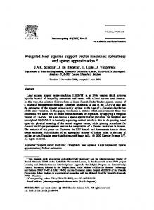
need to be tuned by Bayesian inference. Another hyperparameter is the noise variance σn2 = C1 . As usual, a non-informative prior is assumed for these hyperparameters, and then the likelihood on the hyperparameters becomes the yardstick to choose the optimal values of the hyperparameters. We evaluate the likelihood at two different values of σ 2 in the GPR framework,9 and plot the regression results along with the likelihood value in Figure 1. The negative logarithm of the hyperparameter likelihoods indicate that the Bayesian framework prefers σ 2 = 0.1 to σ 2 = 0.5. For the classifier, the model with σ 2 = 0.1 tends to overfit the training samples. Note that the postprocessing in Van Gestel et al. (2002) cannot be a help for the overfitting result, since it can only adjust the threshold for label prediction. The corresponding results of the standard Gaussian processes for classification with logistic loss function10 (Williams and Barber, 1998) are given for reference in Figure 2, in which the likelihood indicates that the simple model with σ 2 = 0.5 is preferred. Therefore, the use of regression formulation in Bayesian inference for classifier design as did in Van Gestel et al. (2002) might result in the pitfall of overfitting at some unfortunate situations. 7. Conclusion In this paper, we propose an improved scheme of conjugate gradient algorithm for LS-SVM. our scheme will save at least 50% computational expense of the original scheme proposed by Suykens et al. (1999). Comparing with the well-known SMO algorithm described by Keerthi and Shevade (2003), conjugate gradient is relatively suitable to use on medium-size data sets. We also propose an improved scheme for the SMO algorithm for general unconstrained quadratic programming problems. This algorithm is efficient, and quite faster than the standard conjugate gradient on large data sets. As for the Bayesian design for LS-SVM classifiers proposed by Van Gestel et al. (2002), we point out the weakness and illustrate the potential danger of overfitting by a simple example. References Chu, W., S. S. Keerthi, and C. J. Ong. Bayesian support vector regression using a unified loss function. submitted to IEEE transaction of neural networks, 2002. http://guppy.mpe.nus.edu.sg/∼chuwei/paper/ieeebisvr.pdf. Fletcher, R. Practical methods of optimization. John Wiley and Sons, 1987. Keerthi, S. S. and S. K. Shevade. SMO algorithm for least squares SVM formulations. Neural Computation, 15(2), Feb. 2003. Saunders, C., A. Gammerman, and V. Vovk. Ridge regression learning algorithm in dual vari8

Here, N (µ, σ 2 ) is used to denote a Gaussian distribution with the mean µ and the variance σ 2 . The noise variance σn2 is fixed at some reasonable value, say 0.01. 10 Laplacian approximation is used in the evaluation on hyperparameter likelihood. 9

7

ables. In Proceedings of the 15th International Conference on Machine Learning, pages 515– 521, 1998. Smola, A. J. and B. Sch¨olkopf. A tutorial on support vector regression. Technical Report NC2-TR-1998-030, GMD First, October 1998. Steihaug, T. The conjugate gradient method and trust regions in large scale optimization. SIAM Journal of Numerical Analysis, 20(3):626–637, 1983. Suykens, J. A. K., L. Lukas, P. Van Dooren, B. De Moor, and J. Vandewalle. Least squares support vector machine classifiers: a large scale algorithm. In Proc. of the European Conference on Circuit Theory and Design (ECCTD’99), pages 839–842, 1999. Suykens, J. A. K., T. Van Gestel, J. Vanthienen, and B. De Moor. A support vector machine formulation to PCA. ESAT-SCD-SISTA Technical Report 2002-68, Katholieke University Leuven, Leuven, Belgium, 2002. Suykens, J. A. K. and J. Vandewalle. Least squares support vector machine classifiers. Neural processing letters, 9(3):293–300, 1999. Van Gestel, T., J. A. K. Suykens, B. Baesens, S. Viaene, J. Vanthienen, G. Dedene, B. De Moor, and J. Vandewalle. Benchmarking least squares support vector machine classifiers. Internal Report 00-37, ESAT-SISTA, Leuven, Belgium, 2000. Van Gestel, T., J. A. K. Suykens, G. Lanckriet, A. Lambrechts, B. De Moor, and J. Vandewalle. A Bayesian framework for least squares support vector machine classifiers, Gaussian processes and kernel fisher discriminant analysis. Neural Computation, 14:1115–1147, 2002. Vapnik, V. N. The Nature of Statistical Learning Theory. New York: Springer-Verlag, 1995. Williams, C. K. I. and D. Barber. Bayesian classification with Gaussian processes. IEEE Transactions on Pattern Analysis and Machine Intelligence, 20(12):1342–1351, 1998. Williams, C. K. I. and C. E. Rasmussen. Gaussian processes for regression. In Touretzky, D. S., M. C. Mozer, and M. E. Hasselmo, editors, Advances in Neural Information Processing Systems, volume 8, pages 598–604, 1996. MIT Press.

8

Regression with σ2=0.5 and σ2n=0.01

2

1.5

1.5

1

1

L(θ) = 135.5

L(θ) = 100.3

0.5 f(x)

f(x)

0.5 0

0

−0.5

−0.5

−1

−1

−1.5

2

Regression with σ =0.1 and σn=0.01

−4

−2

0 x

2

−1.5

4

−4

−2

0 x

2

4

Figure 1. The graphs of regression results at different values of σ 2 . The dots denotes the training data, and the solid curve is the regression function. L(θ) is the negative logarithm of the hyperparameter likelihood.

Classification with σ2=0.5

Classification with σ2=0.1

2

2

1

1

L(θ)= 14.3

f(x)

f(x)

L(θ)= 12.6 0

0

−1

−1

−2

−2 −4

−2

0 x

2

4

−4

−2

0 x

2

4

Figure 2. The graphs of classification results at different values of σ 2 . The dots denotes the training data, and the solid curve is the discriminant function. L(θ) is the negative logarithm of the hyperparameter likelihood.

9

Table 1. A short description on these benchmark data sets we used in numerical experiments. Data Sets Banana Waveform Image Splice MNIST Computer Activity

Size

Input Dimension

Learning Task

400 400 1300 1000 11739 8192

2 21 18 60 400 21

Binary Classification Binary Classification Binary Classification Binary Classification Binary Classification Regression

Miscellaneous

69 Duplicate Data 21 Duplicate Data Digit 0 vs. Digit 8 Normalized Inputs and Outputs

Table 2. Computational costs for SMO and CG algorithms (α = 0 initialization) on small-size data sets. Kernel denotes the number of kernel evaluations, in which each unit corresponding to 106 evaluations. CPU denotes the CPU time in seconds consumed by the optimization. D(α) denotes the final dual functional (8) at the optimal solution.

Banana Dataset σ 2 = 1.8221 CG

Waveform Dataset σ 2 = 24.5325

SMO

CG

SMO

log10 C

Kernel

CPU

D(α)

Kernel

CPU

D(α)

Kernel

CPU

D(α)

Kernel

CPU

D(α)

-4 -3 -2 -1 0 +1 +2 +3 +4

0.239 0.239 0.398 0.715 1.192 1.986 3.733 7.067 15.563

0.070 0.070 0.111 0.221 0.320 0.592 1.013 2.104 4.616

0.0198 0.197 1.881 15.546 97.232 665.397 5669.293 52687.397 494245.928

0.902 0.825 0.530 0.509 0.710 3.496 31.350 319.759 3306.155

0.290 0.260 0.171 0.160 0.200 1.122 10.054 103.199 1070.269

0.0198 0.197 1.881 15.546 97.232 665.396 5669.291 52687.378 494245.799

0.239 0.239 0.318 0.636 1.192 2.939 7.147 11.514 13.340

0.110 0.090 0.140 0.291 0.560 1.485 3.183 5.327 6.101

0.0176 0.173 1.477 9.398 55.415 304.431 972.925 1428.192 1510.110

0.929 0.910 0.517 0.413 0.557 2.355 10.600 21.774 28.214

0.450 0.441 0.251 0.200 0.250 1.141 5.138 10.575 14.040

0.0176 0.173 1.477 9.398 55.415 304.430 972.925 1428.193 1510.110

Table 3. Computational costs for SMO and CG algorithms (α = 0 initialization) on medium-size data sets. Kernel denotes the number of kernel evaluations, in which each unit corresponding to 106 evaluations. CPU denotes the CPU time in seconds consumed by the optimization. D(α) denotes the final dual functional (8) at the optimal solution.

Image Dataset σ 2 = 2.7183 CG

-4 -3 -2 -1 -0 +1 +2 +3 +4

Splice Dataset σ 2 = 29.9641 SMO

CG

SMO

Kernel

CPU

D(α)

Kernel

CPU

D(α)

Kernel

CPU

D(α)

Kernel

CPU

D(α)

2.532 2.532 4.218 10.962 26.980 70.819 216.667 705.636 2256.850

2.484 3.244 5.408 13.831 34.553 87.832 281.750 914.253 2566.242

0.0635 0.618 5.050 28.671 133.878 574.150 2554.951 11554.666 39458.946

9.301 7.444 5.166 4.833 7.036 33.935 253.361 1910.307 11806.379

6.830 5.367 3.776 3.505 4.997 24.225 187.459 2802.560 17331.135

0.0635 0.618 5.050 28.671 133.878 574.150 2554.950 11554.662 39458.943

0.999 1.498 1.996 3.492 6.483 16.951 35.396 55.834 62.813

2.143 3.215 4.325 7.531 14.001 36.816 77.757 120.547 134.298

0.0499 0.497 4.775 36.459 159.990 309.340 348.659 353.380 353.865

4.726 4.364 2.925 3.120 3.120 5.391 10.767 32.722 119.222

8.262 7.551 5.088 5.408 5.348 9.464 18.697 56.892 207.278

0.0499 0.497 4.775 36.459 159.990 309.340 348.659 353.380 353.866

10

Table 4. Computational costs for SMO and CG algorithms (α = 0 initialization) on large-size data sets. Kernel denotes the number of kernel evaluations, in which each unit corresponding to 106 evaluations. CPU denotes the CPU time in seconds consumed by the optimization. D(α) denotes the final dual functional (8) at the optimal solution. MNIST Dataset σ 2 = 0.0025 CG log10 C -2 -1 0 +1 +2

SMO

Kernel

CPU

D(α)

Kernel

CPU

D(α)

413.302 757.752 1722.135 4064.206 9643.847

5611.010 10284.239 23495.622 56682.010 134222.101

56.136 493.689 2685.667 4965.833 5558.749

401.397 403.956 420.814 669.879 1257.794

3515.685 3540.721 3688.304 5872.334 11027.597

56.136 493.689 2685.668 4965.836 5558.752

Computer Activity σ 2 = 20 CG log10 C -2 -1 0 +1 +2

SMO

Kernel

CPU

D(α)

Kernel

CPU

D(α)

335.438 805.028 1710.666 4662.375 14221.886

423.450 1021.007 2185.105 5880.373 17926.644

19.510 80.608 275.971 1002.054 5453.505

158.590 159.148 220.706 845.302 6382.203

149.785 150.226 207.939 798.177 6028.509

19.510 80.608 275.971 1002.054 5453.501

Table 5. Computational costs for SMO and CG algorithms (α = 0 initialization) on small-size data sets. SMO-ONE denotes the algorithm which chooses only one α for updating at each iteration, while SMO-TWO denotes the algorithm which updates the pair of αiup and αilow . Kernel denotes the number of kernel evaluations, in which each unit corresponding to 106 evaluations. CPU denotes the CPU time in seconds consumed by the optimization. Banana Dataset σ 2 = 1.8221 CG

SMO-TWO

Waveform Dataset σ 2 = 24.5325 SMO-ONE

CG

SMO-TWO

SMO-ONE

log10 C

Kernel

CPU

Kernel

CPU

Kernel

CPU

Kernel

CPU

Kernel

CPU

Kernel

CPU

-4 -3 -2 -1 0 +1 +2 +3 +4

0.401 0.480 0.560 0.879 1.358 2.076 3.752 7.184 14.366

0.040 0.060 0.090 0.180 0.310 0.511 0.981 1.983 4.307

0.231 0.372 0.472 0.475 0.662 3.319 29.275 297.143 3028.185

0.070 0.110 0.130 0.130 0.190 0.921 8.102 82.790 851.583

0.202 0.300 0.412 0.455 0.740 4.107 38.145 375.721 3765.697

0.070 0.090 0.120 0.130 0.211 1.191 11.267 109.648 1103.468

0.401 0.480 0.560 0.720 1.278 2.874 6.226 8.859 9.019

0.070 0.100 0.141 0.220 0.491 1.262 2.855 4.106 4.176

0.372 0.489 0.523 0.427 0.481 1.982 7.942 14.127 15.537

0.160 0.210 0.240 0.190 0.211 0.881 3.535 6.370 7.440

0.253 0.350 0.406 0.376 0.618 2.982 12.188 21.588 23.878

0.110 0.160 0.180 0.170 0.280 1.362 5.559 9.864 10.906

11

Table 6. Computational costs for SMO and CG algorithms (α = 0 initialization) on medium-size data sets. SMOONE denotes the algorithm which chooses only one α for updating at each iteration, while SMO-TWO denotes the algorithm which updates the pair of αiup and αilow . Kernel denotes the number of kernel evaluations, in which each unit corresponding to 106 evaluations. CPU denotes the CPU time in seconds consumed by the optimization.

Image Dataset σ 2 = 2.7183 CG log10 C -4 -3 -2 -1 0 +1 +2 +3 +4

Splice Dataset σ 2 = 29.9641

SMO-TWO

SMO-ONE

CG

SMO-TWO

SMO-ONE

Kernel

CPU

Kernel

CPU

Kernel

CPU

Kernel

CPU

Kernel

CPU

Kernel

CPU

4.227 5.071 6.760 12.670 24.491 58.265 160.432 484.662 1477.618

1.001 1.582 2.623 6.119 12.729 34.109 95.999 287.456 873.074

2.383 3.719 4.276 4.370 5.883 25.674 172.959 1167.791 6216.106

2.063 3.415 3.705 3.725 5.939 24.696 160.232 1075.457 5215.521

2.213 3.110 4.320 4.274 5.959 26.372 179.828 1233.935 6648.647

2.804 4.166 5.658 5.238 7.611 32.116 230.143 1604.754 8812.740

2.002 2.502 3.001 4.000 6.498 12.991 18.486 23.980 24.480

1.072 2.173 3.325 5.498 10.826 24.485 36.914 48.019 49.522

1.037 1.567 2.103 2.939 2.745 3.990 5.247 4.614 4.690

1.792 2.754 3.675 5.028 4.717 6.810 9.043 7.901 8.102

1.002 1.416 2.075 2.763 2.866 4.363 5.662 5.257 5.298

2.795 3.886 5.908 7.812 7.762 11.797 15.242 14.230 14.361

Table 7. Computational costs for SMO and CG algorithms (α = 0 initialization) on large-size data sets. SMO-ONE denotes the algorithm which chooses only one α for updating at each iteration, while SMO-TWO denotes the algorithm which updates the pair of αiup and αilow . Kernel denotes the number of kernel evaluations, in which each unit corresponding to 106 evaluations. CPU denotes the CPU time in seconds consumed by the optimization. MNIST Dataset σ 2 = 0.0025 CG log10 C -4 -3 -2 -1 0 +1 +2

SMO-TWO

SMO-ONE

Kernel

CPU

Kernel

CPU

Kernel

CPU

344.528 413.424 482.320 620.113 1171.282 2411.414 4547.196

1894.643 2827.175 3770.051 5653.069 13196.125 30606.006 60751.616

138.526 145.711 152.238 143.645 141.015 167.476 239.040

1209.511 1272.032 1328.934 1253.585 1230.883 1462.067 2086.932

137.734 144.308 151.844 144.096 147.360 210.539 371.645

1969.382 2027.125 2133.530 2024.261 2070.027 2957.382 5222.142

Computer Activity σ 2 = 20 CG log10 C -4 -3 -2 -1 0 +1 +2

SMO-TWO

SMO-ONE

Kernel

CPU

Kernel

CPU

Kernel

CPU

201.335 234.885 369.086 704.590 1409.147 3623.469 10199.335

127.303 169.023 339.488 764.619 1643.703 4420.697 12697.277

156.247 164.555 146.138 132.358 174.418 685.876 4886.482

143.107 150.456 134.734 121.645 160.371 629.094 4542.462

123.716 144.515 140.993 132.964 241.140 1321.066 11074.888

171.787 200.609 196.112 185.477 335.923 1840.186 15429.912

12