A New Least Squares Support Vector Machines Ensemble Model for ...

Hindawi Publishing Corporation Mathematical Problems in Engineering Volume 2016, Article ID 4615903, 8 pages http://dx.doi.org/10.1155/2016/4615903

Research Article A New Least Squares Support Vector Machines Ensemble Model for Aero Engine Performance Parameter Chaotic Prediction Dangdang Du, Xiaoliang Jia, and Chaobo Hao School of Mechanical Engineering, Northwestern Polytechnical University, Xi’an 710072, China Correspondence should be addressed to Xiaoliang Jia; [email protected] Received 25 September 2015; Accepted 26 January 2016 Academic Editor: Francesco Franco Copyright © 2016 Dangdang Du et al. This is an open access article distributed under the Creative Commons Attribution License, which permits unrestricted use, distribution, and reproduction in any medium, provided the original work is properly cited. Aiming at the nonlinearity, chaos, and small-sample of aero engine performance parameters data, a new ensemble model, named the least squares support vector machine (LSSVM) ensemble model with phase space reconstruction (PSR) and particle swarm optimization (PSO), is presented. First, to guarantee the diversity of individual members, different single kernel LSSVMs are selected as base predictors, and they also output the primary prediction results independently. Then, all the primary prediction results are integrated to produce the most appropriate prediction results by another particular LSSVM—a multiple kernel LSSVM, which reduces the dependence of modeling accuracy on kernel function and parameters. Phase space reconstruction theory is applied to extract the chaotic characteristic of input data source and reconstruct the data sample, and particle swarm optimization algorithm is used to obtain the best LSSVM individual members. A case study is employed to verify the effectiveness of presented model with real operation data of aero engine. The results show that prediction accuracy of the proposed model improves obviously compared with other three models.

1. Introduction With increasing demands in the field of operation safety, asset availability, and economy, the health monitoring of aero engine has been widely considered as the key prerequisite for the competition of an airline company. One of the main tasks of health monitoring is to predict the performance parameter of aero engine. By predicting and analyzing the trend of performance parameters, one can obtain valuable information to avoid future risk and loss due to faults or accidents and reduce associated maintenance costs [1]. Therefore, it is necessary to design a high accurate and robust prediction model for aero engine performance parameter (AEPP). A variety of traditional time series prediction approaches have already been proposed for this problem, such as fuzzy rule [2], Kalman filter [3], grey prediction [4], ARMA [5], and multiple regression [6]. These approaches are very mature in theory, but the accuracy is not always high and the robustness is not always satisfied in the application [7]. With the development of artificial intelligence techniques, recent

studies for AEPP prediction are mainly focused on artificial neural network (ANN) [8, 9] and support vector machine (SVM) [10, 11]. Compared with standard SVM, least squares support vector machine (LSSVM) adopts equality constraints and a linear Karush-Kuhn-Tucker system, which has a more powerful computational ability in solving the nonlinear and smallsample problem [12, 13]. In addition, LSSVM eliminates local minima and structure design complexity of ANN. Therefore, LSSVM is a good choice for AEPP prediction model designing. However, the modeling accuracy of a single LSSVM is not only influenced by the input data source, but also affected by its kernel function and regularization parameters [12]. Thus, several main disadvantages are worth to be addressed. Firstly, using a data-driven technique to design an LSSVM model, data source should be considered as the first factor. AEPP data is different from the pure random system: that is, the chaotic characteristic of AEPP data should be extracted to reconstruct input data samples before modeling. Secondly, as two common parameter optimized methods for LSSVM,

2 conventional cross-validation and grid search methods have several defects, such as high time consuming and a priori knowledge requirement. In addition, although a single LSSVM with optimal parameters and reconstructed input data samples may have an excellent prediction performance under certain circumstances, because its kernel function is fixed, it perhaps has some kinds of inherent bias under other cases. In the literatures, due to the super robustness and generalization, ensemble model has been proved to be an effective way to reduce biases of single model. Ensemble model can make full use of diversity to compensate for disadvantages among the individual members, and the reasonable combination strategy is believed to be able to produce better prediction accuracy and generalization than single model [13–16]. By using combining submodels, the multilayer networks of LS-SVMs ensemble have been discussed deeply, which is very encouraging and promising for further research [13], but up to now, the application of LSSVM ensemble model for AEPP prediction is relatively fresh and untouched in the open literature. For ensemble model design, there are two points that should be considered. One is that the selected individual members need to exhibit much diversity (disagreement) and accuracy. The other is the effectiveness of the combination strategy [17]. For the diversity of individual members, it is an easy and common way to build individual members by using data decomposition [18]. However, this method is proved to be effective when the original data sample is sufficient, and it is not suitable for small-sample data. Compared with the existing combination strategies such as simple averaging weighting method, mean squared error weighting method, and least squares estimation weighting averaging method, intelligent method based combination strategies include ANN combiner and SVM combiner which have become the current trend [18]; however, ANN combiner cannot avoid falling into local optima, and for SVM combiner it is not easy to select appropriate kernel function, so it is necessary to further improve these ensemble strategies. As previously mentioned, in this paper, a new PSRPSO-(SK)LSSVM-(MK)LSSVM ensemble (PPLLE) model for AEPP prediction is proposed. Firstly, a set of diverse single kernel LSSVMs are created as base predictors. Subsequently these individual member LSSVMs output the primary prediction results independently. Finally, all the primary prediction results are combined to produce the most appropriate prediction results by another particular multiple kernel LSSVM. In the process of modeling, phase space reconstruction (PSR) theory is applied to extract the chaotic characteristic of input data source and reconstruct the data samples. Particle swarm optimization algorithm is used to search the best parameters for LSSVM members to ensure their prediction accuracies. The rest of this paper is organized as follows. The next section provides a brief introduction to the related knowledge. Section 3 formulates the proposed PPLLE model. For illustration purpose, the detailed application on AEPP prediction and model comparisons is proposed in Section 4. Section 5 concludes this study.

Mathematical Problems in Engineering

2. An Overview of the Related Knowledge 2.1. Data Samples Reconstruction Based on PSR Theory. Although the nonlinear chaos behavior is the main challenge confronting the chaotic data series prediction, the underlying data generating mechanisms can still be explored by PSR theory [19]. By means of the ability of revealing the nature of dynamic system state, the PSR theory is useful in system characterization, in nonlinear prediction, and in estimating bounds on the size of the system [20, 21]. According to Takens’ theorem, for the nonlinear time series {𝑥𝑖 }𝑛𝑖=1 , the current state information can be represented by an 𝑚-dimensional vector: 𝑥𝑖+𝜏 = 𝑓 (𝑥𝑖 , 𝑥𝑖−𝜏 , . . . , 𝑥𝑖−(𝑚−1)𝜏 ) ,

(1)

where 𝜏 is the delay time, 𝑚 is the embedded dimension, they are two important parameters for phase space construction, and 𝑓 is the mapping relation between the inputs and outputs. The autocorrelation function of time series at the first minimum value is taken as the delay time 𝜏 of the reconstructed phase space; we write CR =

∑𝑛−𝜏 𝑖=1 (𝑥𝑖 − 𝑥) (𝑥𝑖+𝜏 − 𝑥) 2

∑𝑛−𝜏 𝑖=1 (𝑥𝑖 − 𝑥)

,

(2)

where 𝑥 is the mean of 𝑥𝑖 . To calculate the correlation dimension, the correlation integral 𝐶(𝑟) needs to be computed: 𝐶 (𝑟) =

1 𝑁 𝑁 󵄩 󵄩 ∑ ∑ 𝑢 (𝑟 − 󵄩󵄩󵄩󵄩𝑋𝑖 − 𝑋𝑗 󵄩󵄩󵄩󵄩) , 𝑁2 𝑖=1 𝑗=1

(3)

where 𝑟 is the selected radius and 𝑟 > 0, 𝑢(𝑥) is the Heaviside function. The correlation dimension 𝑑(𝑚) is calculated by the formula as below: 𝑑 (𝑚) =

ln 𝐶 (𝑟) . ln 𝑟

(4)

Suppose 𝑌𝑖 = 𝑥𝑖 , 𝑋𝑖 = (𝑥𝑖−𝜏 , 𝑥𝑖−2𝜏 , . . . , 𝑥𝑖−𝑚𝜏 ); then we can reconstruct 𝑛 − 𝑚 data samples {𝑋𝑖 , 𝑌𝑖 }𝑛𝑚+1 . 2.2. Least Squares Support Vector Machine. LSSVM is the least squares form of a standard SVM; it was firstly proposed by Suykens and Vandewalle [12]. LSSVM uses a set of linear equations during the training process and chooses all training data as support vectors, so it has excellent generalization and low computation complexity [12–14]. In LSSVM, the regression issue can be expressed as the following optimization problem: min

1 𝑁 1 ‖𝑊‖2 + 𝛾∑𝑒𝑡2 2 2 𝑡=1

(𝛾 > 0)

(5)

s.t. 𝑦𝑡 = ⟨𝑊, 𝜑 (X𝑡 )⟩ + 𝑏 + 𝑒𝑡 , where 𝜑(X𝑡 ) is a nonlinear function which maps the input data into a higher dimensional space. 𝑒𝑡 is the error at time 𝑡, 𝑏 is the bias, and 𝛾 is the regulation constant.

Mathematical Problems in Engineering

3

According to the Lagrange function and Karush-KuhnTucker theorem, the LSSVM for nonlinear functions can be given as below: 𝑁

𝑦𝑡 = ∑𝛼𝑡 𝐾 (𝑋, 𝑋𝑡 ) + 𝑏,

(6)

𝑡=1

where 𝛼𝑡 is the Lagrange multiplier and 𝐾(𝑋, 𝑋𝑡 ) is the kernel function which is applied to substitute the mapping process and avoid computing the function 𝜑(X𝑡 ). Typical kernel functions include linear kernel function, polynomial kernel function, radial basis kernel function, sigmoid kernel function, and multiple kernel function. Some of them are listed as follows: (1) linear kernel function (LKF): 𝐾 (𝑋, 𝑋𝑡 ) = (𝑋, 𝑋𝑡󸀠 ) ,

(7)

𝑞

(3) Gaussian radial basis kernel function (RBF): 󵄩2 󵄩󵄩 󵄩𝑋 − 𝑋𝑡 󵄩󵄩󵄩 ), 𝐾 (𝑋, 𝑋𝑡 ) = exp (− 󵄩 𝜎2

(8)

(9)

(4) sigmoid kernel function (SKF): 𝐾 (𝑋, 𝑋𝑡 ) = tanh (] (𝑋, 𝑋𝑡 ) + 𝑒) ,

(10)

(5) multiple kernel function (MKF): 𝐾 (𝑋, 𝑋𝑡 ) = 𝜌1 𝐾1 (𝑋, 𝑋𝑡 ) + ⋅ ⋅ ⋅ + 𝜌𝑛 𝐾𝑛 (𝑋, 𝑋𝑡 ) 𝑛

s.t.

∑𝜌𝑖 = 1 𝑖=1

(0 ≤ 𝜌𝑖 ≤ 1) .

𝑡+1 𝑡 𝑡 𝑡 𝑡 𝑡 = [𝜔V𝑖𝑑 + 𝑐1 𝑟1 (𝑝𝑖𝑑 − 𝑥𝑖𝑑 ) + 𝑐2 𝑟2 (𝑝𝑔𝑑 − 𝑥𝑖𝑑 )] , V𝑖𝑑 𝑡+1 𝑡 𝑡+1 = 𝑥𝑖𝑑 + V𝑖𝑑 , 𝑥𝑖𝑑

(2) polynomial kernel function (PKF): 𝐾 (𝑋, 𝑋𝑡 ) = [(𝑋, 𝑋𝑡 ) + 1] ,

2.3. Parameters Optimized Based on PSO. Particle swarm optimization (PSO) algorithm is a popular swarm intelligence evolutionary algorithm used for solving global optimization problem [22]. It can search the global optimal solution in different regions of the solution space in parallel. In PSO, the position of each particle represents a solution to the optimization problem. 𝑥𝑘 = (𝑥𝑘1 , 𝑥𝑘2 , . . . , 𝑥𝑘𝑑 ) is the position vector and V𝑘 = (V𝑘1 , V𝑘2 , . . . , V𝑘𝑑 ) is the velocity vector of the 𝑘th particle. Similarly, 𝑃𝑘 = (𝑝𝑘1 , 𝑝𝑘2 , . . . , 𝑝𝑘𝑑 ) represents the best position of the 𝑘th particle which has been achieved, and 𝑃𝑔 = (𝑝𝑔1 , 𝑝𝑔2 , . . . , 𝑝𝑔𝑑 ) represents the best position among the whole particle group. The values of position and velocity of the particle are updated as follows:

(11)

The nonlinear mapping ability of LSSVM is mainly determined by its kernel function form and relevant parameters setting: that is, various kernel functions or parameters have different influence on the prediction ability of LSSVM predictor (the parameters setting will be discussed in the next section). As to kernel function, the LKF is suited to expressing the linear component of the mapping relation, and the RBF possesses a wider convergence domain and an outstanding learning ability and high resolution power, while the PKF has a powerful approximation and generalization ability. Meanwhile, kernel functions can also be divided into local kernel function and global kernel function. For the global kernel function, it has the overall situation characteristic and is commonly good at fitting the sample points which are far away from the testing points, but the fitting effect is not perfect on the sample points which are near the testing points, and vice versa to the local kernel function [15]. Each kind of kernel function has its own advantages and disadvantages; the prediction performances of LSSVM with different kernel functions are not identical. Here, we define the LSSVM configured with a multiple kernel function as the multiple kernel LSSVM (MK-LSSVM); otherwise, we call it the single kernel LSSVM (SK-LSSVM).

(12)

where 𝑐1 and 𝑐2 are the acceleration constant, 𝑟1 and 𝑟2 are two random numbers in the range [0, 1], and 𝜔 is inertia weight factor. To improve the convergence speed of PSO, 𝑐1 , 𝑐2 , and 𝜔 of PSO are adjusted by using the formulas as below: 𝜔 = 𝜔max −

𝜔max − 𝜔min 𝑡, 𝑡max

𝑐1 = 𝑐1max −

𝑐1max − 𝑐1min 𝑡, 𝑡max

𝑐2 = 𝑐2max −

𝑐2max − 𝑐2min 𝑡, 𝑡max

(13)

where 𝑡max expresses the maximum iteration number and 𝑡 is the current iteration number.

3. Overall Process of Designing the PPLLE Model The core idea of the ensemble model lies in that all the individual members are accurate as much as possible and diverse enough, and it adopts an appropriate ensemble strategy to combine these outputs of the selected members [13–18]. 3.1. Selection of the Appropriate Individual Member Predictors. For LSSVM prediction model, several diverse strategies, such as data diversity, parameter diversity, and kernel diversity, have been proved effectively for the creation of ensemble members with much dissimilarity [13]. Because kernel function has a crucial and direct effect on the learning and generalizing performance of LSSVM, various kernel functions can be used to create diverse LSSVMs. In this study, 𝑛 independent SK-LSSVMs, such as LKF-LSSVM, PKFLSSVM, and RBF-LSSVM, are selected as individual member LSSVM predictors. 3.2. Combination of the Selected Individual Member LSSVM Predictors. After the diverse individual member LSSVM

4

Mathematical Problems in Engineering Stage 1

Stage 2

Here, 𝑓(⋅) is the mapping function determined by the special combiner MK-LSSVM; thus, the final prediction ̂ of the PPLLE model can be given as below: output 𝑦

Stage 3

Individual ̂1 SK-LSSVM1 x Data source PSR

̂2, 𝑥 ̂3, . . . , 𝑥 ̂𝑛) . ̂ = 𝑓 (̂ 𝑦 𝑥1 , 𝑥

Individual x ̂2 SK-LSSVM2

Reconstruct data samples ···

···

Combiner MK-LSSVM

̂ y

̂n x

Partition data samples Individual SK-LSSVMn

PSO

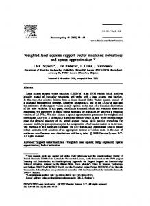
Figure 1: Basic framework of the PPLLE model.

predictors have been selected, the other key question is how to determine the weight coefficient of each individual predictor, that is, how to construct the combiner effectively. As depicted in previous section, the MKF integrates the advantages of global kernel function and local kernel function and offsets some shortages of both simultaneously. Hence, another special MK-LSSVM is chosen as the combiner. In this paper, the MKF is composed of a RBF and a PKF: the former is a typical local kernel function and the latter is a representative globe kernel function. A similar MK-LSSVM model has high prediction accuracy and generalization ability, which has been proved with chaotic time series by Tian et al. [15]. 3.3. Overall Process of Designing the PPLLE Model. The basic framework of the proposed PPLLE model is given in Figure 1, where 𝑛 is the number of the individual member LSSVM predictors. As shown in Figure 1, there are three main stages in the basic framework which can be summarized as follows. Stage 1 (sample dataset reconstruction and partition). The data source is reconstructed as data samples by using PSR; then the reconstructed data samples are divided into two indispensable subsets: training subset and testing subset. Stage 2 (individual member creation and prediction). Based on kernel function diversity principle, 𝑛 independent SKLSSVMs are created as the individual member. Each SKLSSVM is trained by using the training subset. Accordingly, ̂2, 𝑥 ̂3, . . . , 𝑥 ̂ 𝑛 of the 𝑛 SK̂1, 𝑥 the computational results 𝑥 LSSVM predictors can be obtained, respectively. In the process of SK-LSSVM creating, PSO is used to optimize parameters of each member SK-LSSVM. Stage 3 (combiner creation and prediction). When the computational results of the individual member predictors in the second stage are acquired, they are aggregated into an ensemble result by another special MK-LSSVM. Similarly, to create the optimal MK-LSSVM, PSO is applied again.

(14)

4. Case Study Due to different gas path component degradations such as fouling, erosion, corrosion, and foreign object damage, the performance of an aero engine will decline over the service time [23]. A lot of gas path performance parameters are often used in health monitoring of aero engine from different angles and levels, such as exhaust gas temperature (EGT), fuel flow (FF), and low pressure fan speed (N1). Among these performance parameters, EGT is considered as one of the most crucial working performance parameters of aero engine, which is measured to represent outlet temperature of combustor chamber in practice. When other conditions remain the same, the higher the EGT is, the more serious the performance degradation of aero engine is [4]. EGT gradually rises when the working life of aero engine increases, if the EGT value reaches or exceeds the scheduled threshold provided by the original equipment manufacturer, then the aero engine needs to be arranged for maintenance timely. In this study, we select EGT as the AEPP representative to predict by using the proposed PPLLE model, and it is worth mentioning that other similar parameters can also be predicted in the same way. 4.1. Data Description and Samples Reconstruction. In this study, the EGT data come from the real flight recorders of the cruise state of a certain type of aero engine, and the sampling interval is 5 flight cycles. The data series consists of 148 EGT datasets, covering the period from February 2013 to September 2014. To increase the quality of the prediction results, some abnormal samples have been discarded from the original data series. The observed EGT data is shown in Figure 2. For the observed EGT data series {EGT𝑖 }148 𝑖=1 , according to (2), (3), and (4), the delay time 𝜏 is set as 1 and embedding dimension 𝑚 = 5 is obtained by computing. Thus, (EGT𝑖−5 , EGT𝑖−4 , . . . , EGT𝑖−1 ) is taken as the input vector 𝑋𝑖 , and 𝑌𝑖 = EGT𝑖 (𝑖 = 6, 7, . . . , 148) is used as the corresponding expected value, so we can get the reconstructed data samples 120 {𝑋𝑖 , 𝑌𝑖 }148 𝑖=6 . The data samples {𝑋𝑖 , 𝑌𝑖 }𝑖=6 are used as training subset to train each individual LSSVM of the ensemble model, and the samples {𝑋𝑖 , 𝑌𝑖 }148 𝑖=121 are chosen as testing subset to validate the ensemble model. The one-step ahead prediction used in this paper is explained as in Figure 3. After the ensemble model has been trained, vector 𝑋121 is entered into 4 individual predictors (SK-LSSVM prediĉ 2121 , . . . , 𝑥 ̂ 4121 , ̂ 1121 , 𝑥 tors) to compute their predicted values 𝑥 respectively. Then, these predicted values are aggregated into an ensemble result by using a combination predictor (MK̂ 121 is LSSVM predictor). Hence, the final predicted value 𝑦 obtained. In this way, from 𝑖 = 121 to 148, all the final ̂ 148 can be got in turn. ̂ 121 to 𝑦 predicted values 𝑦

Mathematical Problems in Engineering

5

Table 1: Optimal parameters of LSSVM2 ∼LSSVM5 . LSSVM2 (PKF-LSSVM) 𝑞=3 𝛾 = 93.41

LSSVM1 (LKF-LSSVM)

LSSVM3 (RBF-LSSVM) 𝜎2 = 0.32 𝛾 = 176.82

LSSVM4 (SKF-LSSVM) V = 1, 𝑒 = 1 𝛾 = 125.13

750

LSSVM5 (MK-LSSVM) 𝑞 = 2, 𝜎2 = 0.51 𝜌 = 0.27, 𝛾 = 168.3

i = 121

740

i= i+1

i > 148

No

End

Yes EGT (∘ C)

730

Individual predictor1

720 Xi

710

̂ 2i x ···

···

700 690

Individual predictor2

̂ 1i x

Combination predictor

̂i y

̂ 4i x

Individual predictor4

Figure 3: One-step ahead prediction from 𝑖 = 121 to 148.

0 10 20 30 40 50 60 70 80 90 100 110 120 130 140 150 Sample number

750

Observed data

Figure 2: The observed EGT data. 740

700

1 𝑘 󵄨󵄨 ̂ 𝑖 󵄨󵄨󵄨󵄨 , ∑ 󵄨𝑦 − 𝑦 𝑘 𝑖=1 󵄨 𝑖

690 120

TIC =

2 √∑𝑘𝑖=1 (𝑦𝑖 )2 + √∑𝑘𝑖=1 (̂ 𝑦𝑖 )

125

130

135 140 Sample number

145

150

(15)

1 𝑘 2 ̂𝑖) , MSE = ∑ (𝑦𝑖 − 𝑦 𝑘 𝑖=1 2 √∑𝑘𝑖=1 (𝑦𝑖 − 𝑦 ̂𝑖)

720 710

̂ 𝑖 󵄨󵄨󵄨 1 󵄨󵄨󵄨 𝑦 − 𝑦 󵄨󵄨 × 100, MAPE = ∑ 󵄨󵄨󵄨 𝑖 𝑘 𝑖=1 󵄨󵄨 𝑦𝑖 󵄨󵄨󵄨 𝑘

MAE =

730 EGT (∘ C)

4.2. Evaluation Indices. Mean absolute percentage error (MAPE), mean absolute error (MAE), mean squared error (MSE), and Theil’s Inequality Coefficient (TIC) are used to evaluate the prediction ability of the prediction model:

Observed data PPLLE predicted data

,

̂ 𝑖 are the observed values and corresponding where 𝑦𝑖 and 𝑦 prediction values, respectively. 4.3. Model Parameters Setting. In the modeling process of LSSVMs, the parameters of PSO are set as follows: 𝑐1min = 𝑐2min = 2, 𝑐1max = 𝑐2max = 3, 𝜔min = 1, 𝜔max = 3, 𝑝 = 50, and 𝑡max = 1000. By using the PSO, the corresponding optimal parameters of LSSVM2 ∼LSSVM5 are obtained and listed in Table 1. An appropriate individual member number of the ensemble model is able to achieve a balance between

Figure 4: Prediction results of the PPLLE model on EGT testing dataset.

the prediction efficiency and the prediction ability [17]. In this study, the member number is set as 5. 4.4. Results and Discussion. Figure 4 illustrates the prediction results for the EGT testing dataset by PPLLE model and corresponding observed EGT value. The black symbol represents the observed value, and the red symbol expresses the prediction value. From Figure 4, we can find that the rise and fall trends of the two curves are approximately the same, and only the individual points have some higher gaps of the size, which means EGT is predicted with good

6

Mathematical Problems in Engineering 750

Table 2: Comparison of different models on EGT testing dataset. MAPE (%) 0.51 0.62 0.85 1.10

MAE 3.67 4.48 6.16 7.99

MSE 14.04 22.48 49.70 75.66

TIC 0.00258 0.00327 0.00485 0.00598

accuracy on the testing data samples as a whole. There are two causes that may explain the gaps between the observed values and prediction values. Firstly, it is difficult to give a thorough consideration to extract the EGT characteristics when determining the model input data. Secondly, due to the influence of subjective factors, it is impossible to eliminate all the outliers properly. In contrast, the single LSSVM model proposed by Tian et al. [15], RBF-chaos model proposed by Zhang et al. [24], and PPLLE∗ (PSR-PSO-LSSVM-LSSVM∗ ensemble) model are built. The kernel function and parameters of the single LSSVM model are the same as those of the LSSVM5 model listed in Table 1. The RBF-chaos model aggregated chaos characteristics and RBF neural networks (here, the input layer, hidden layer, and output layer of RBF neural network are set as 5, 11, and 1, resp.). The difference between the PPLLE model and PPLLE∗ model lies in that the latter uses an RBFLSSVM (i.e., SK-LSSVM) as the combiner. In Table 2, the MAPE, MAE, MSE, and TIC values of the PPLLE, PPLLE∗ , RBF-chaos, and single LSSVM models on the testing dataset are listed. It shows that the PPLLE model performs the best among the four modes with MAPE of 0.51, compared with those of 0.62, 0.85, and 1.10 by the PPLLE∗ , RBF-chaos, and single LSSVM models, respectively. The MAE of PPLLE, PPLLE∗ , RBF-chaos, and single LSSVM models are 3.67, 4.48, 6.16, and 7.99, respectively, which demonstrates the prediction accuracy of the proposed model. PPLLE model predicts the EGT with MSE of 14.04, better than PPLLE∗ , RBF-chaos, and single LSSVM models with those of 22.48, 49.70, and 75.66, respectively. Besides, it should be pointed out that the TIC of PPLLE is 0.00258, which is quite acceptable compared with those of the other 3 models. A strong support is also exhibited by Figure 5, where the curve of PPLLE model intuitively shows the good prediction accuracy and excellent ability in tracking the observed EGT compared to the other 3 models. Figures 6(a)–6(d) show a detailed profile of relative percentage error (RPE) between the observed values and prediction values of different models on the EGT testing data samples. It illustrates that the PPLLE model has an outstanding approximation ability with the RPE ranging from −0.7% to 0.9%; the RPE ranging around [−1.4%, 2.9%] in Figure 6(d) shows that the single LSSVM has the worst performance. RPE distribution range of PPLLE∗ model is better than that of RBF-chaos model, which are exhibited by Figures 6(c) and 6(d). Comparison results of Figure 6 also prove the effectiveness of our proposed approach. Some of the main reasons why the PPLLE model is superior to others can be summarized as follows: (1) the PPLLE ensemble model based on kernel diverse principle eliminates

740 730 EGT (∘ C)

Model PPLLE PPLLE∗ RBF-chaos Single LSSVM

720 710 700 690 120

125

130

135

140

145

150

Sample number Observed data PPLLE predicted data PPLLE∗ predicted data

RBF-chaos predicted data Single LSSVM predicted data

Figure 5: Prediction results of different models on EGT testing dataset.

the possible inherent biases of single LSSVM and makes full use of the advantages of individual member LSSVMs; (2) the PSR extracts the chaotic feature of the original data source and reconstructs data samples, which elucidates the input characteristic for the PPLLE model; (3) the PSO ensure that each individual LSSVM achieves the best performance; (4) the particular ensemble strategy of PPLLE employs an MKLSSVM and further enhances the prediction ability of the ensemble model.

5. Conclusions Designing a high accuracy and robust model for AEPP prediction is quite challenging, since AEPP data is nonlinear, chaotic, and small-sample, and the traditional single prediction model may have some inherent biases. To solve this problem and to realize high prediction accuracy level, a new LSSVM ensemble model based on PSR and PSO is presented and applied to AEPP prediction in this paper. For the presented PPLLE prediction model, individual member LSSVMs based on kernel diverse principle eliminate the inherent biases of single LSSVM and make full use of the advantages of them as much as possible. PSR is applied to reconstruct data samples, which alleviates the influence of the chaotic feature of the original data source to the PPLLE model. PSO is used to guarantee that each individual LSSVM achieves the best performance. The particular ensemble strategy employs an MK-LSSVM combiner, as the MKF integrates the advantages of global kernel function and local kernel function, and it offsets some shortages of both; this ensemble strategy further enhances the prediction ability of the ensemble model. EGT is selected as the representative health monitoring parameter of aero engine for validating the effectiveness of the

7

3

3

2

2

1

1 EGT RPE

EGT RPE

Mathematical Problems in Engineering

0

0

−1

−1

−2

−2

−3 120

125

130

135 140 Sample number

145

−3 120

150

125

3

3

2

2

1

1 EGT RPE

EGT RPE

145

150

145

150

(b) RPE of PPLLE∗

(a) RPE of PPLLE

0

0

−1

−1

−2

−2

125

135 140 Sample number

PPLLE∗

PPLLE

−3 120

130

130

135 140 Sample number

145

150

−3 120

125

130

135 140 Sample number

Single LSSVM

RBF-chaos (c) RPE of RBF-chaos

(d) RPE of single LSSVM

Figure 6: RPE comparison of different models on EGT testing dataset.

proposed PPLLE model. For comparison, the PPLLE∗ , RBFchaos, and single LSSVM models are also developed and evaluated. The PPLLE predicts EGT with MAPE of 0.51%, better than the PPLLE∗ , RBF-chaos, and single LSSVM models with those of 0.62%, 0.85%, and 1.10%, respectively. Similarly, the PPLLE predicts EGT with TIC of 0.00258, better than the PPLLE∗ , RBF-chaos, and single LSSVM models with those of 0.00327, 0.00485, and 0.00598, respectively. In addition, MAE and MSE indices also confirm that the presented model gives improved prediction accuracy. In a word, the above four evaluation indices consistently demonstrate that the PPLLE model is more suitable for AEPP prediction problem, and the PPLLE model can meet the actual demand of engineering application. Moreover, comparing results imply that this ensemble model has a promising application in other similar engineering areas where the data have complex nonlinear chaos relationships.

Conflict of Interests The authors declare that there is no conflict of interests regarding the publication of this paper.

References [1] L.-F. Yang and I. Ioachim, “Adaptive estimation of aircraft flight parameters for engine health monitoring system,” Journal of Aircraft, vol. 39, no. 3, pp. 404–408, 2002. [2] J. Hong, L. Han, X. Miao et al., “Fuzzy logic inference for predicting aero-engine bearing grad-life,” in Proceedings of the 9th International Flins Conference on Computational Intelligence: Foundations and Applications, vol. 4, pp. 367–373, Chengdu, China, August 2010. [3] G. You and N. Wang, “Aero-engine condition monitoring based on Kalman filter theory,” Advanced Materials Research, vol. 490– 495, no. 4, pp. 176–181, 2012.

8 [4] N.-B. Zhao, J.-L. Yang, S.-Y. Li, and Y.-W. Sun, “A GM (1, 1) Markov chain-based aeroengine performance degradation forecast approach using exhaust gas temperature,” Mathematical Problems in Engineering, vol. 2014, Article ID 832851, 11 pages, 2014. [5] Z. G. Liu, Z. J. Cai, and X. M. Tan, “Forecasting research of aeroengine rotate speed signal based on ARMA model,” Procedia Engineering, vol. 15, pp. 115–121, 2011. [6] Y.-X. Song, K.-X. Zhang, and Y.-S. Shi, “Research on aeroengine performance parameters forecast based on multiple linear regression forecasting method,” Journal of Aerospace Power, vol. 24, no. 2, pp. 427–431, 2009 (Chinese). [7] C. Chatfield, The Analysis of Time Series: An Introduction, Chapman & Hall/CRC, Boca Raton, Fla, USA, 6th edition, 2003. [8] S. G. Luan, S. S. Zhong, and Y. Li, “Hybrid recurrent process neural network for aero engine condition monitoring,” Neural Network World, vol. 18, no. 2, pp. 133–145, 2008. [9] D. Gang and S. S. Zhong, “Aircraft engine lubricating oil monitoring by process neural network,” Neural Network World, vol. 16, no. 1, pp. 15–24, 2006. [10] C. Zhang and N. Wang, “Aero-engine condition monitoring based on support vector machine,” Physics Procedia, vol. 24, pp. 1546–1552, 2012. [11] X.-Y. Fu and S.-S. Zhong, “Aeroengine turbine exhaust gas temperature prediction using process support vector machines,” in Advances in Neural Networks—SNN 2013, vol. 7951 of Lecture Notes in Computer Science, pp. 300–310, Springer, Berlin, Germany, 2013. [12] J. A. K. Suykens and J. Vandewalle, “Least squares support vector machine classifiers,” Neural Processing Letters, vol. 9, no. 3, pp. 293–300, 1999. [13] J. A. K. Suykens, T. Van Gestel, J. De Brabanter, B. De Moor, and J. Vandewalle, Least Squares Support Vector Machines, World Scientific, Singapore, 2002. [14] X. Yan and N. A. Chowdhury, “Mid-term electricity market clearing price forecasting: a hybrid LSSVM and ARMAX approach,” International Journal of Electrical Power & Energy Systems, vol. 53, no. 1, pp. 20–26, 2013. [15] Z.-D. Tian, X.-W. Gao, and T. Shi, “Combination kernel function least squares support vector machine for chaotic time series prediction,” Acta Physica Sinica, vol. 63, no. 16, Article ID 160508, 2014 (Chinese). [16] O. Cagcag Yolcu, “A hybrid fuzzy time series approach based on fuzzy clustering and artificial neural network with single multiplicative neuron model,” Mathematical Problems in Engineering, vol. 2013, Article ID 560472, 9 pages, 2013. [17] L. Yu, W. Y. Yue, S. Y. Wang, and K. K. Lai, “Support vector machine based multiagent ensemble learning for credit risk evaluation,” Expert Systems with Applications, vol. 37, no. 2, pp. 1351–1360, 2010. [18] Y. Lv, J. Liu, T. Yang, and D. Zeng, “A novel least squares support vector machine ensemble model for NO𝑥 emission prediction of a coal-fired boiler,” Energy, vol. 55, pp. 319–329, 2013. [19] Q. Zhang, P. W.-T. Tse, X. Wan, and G. Xu, “Remaining useful life estimation for mechanical systems based on similarity of phase space trajectory,” Expert Systems with Applications, vol. 42, no. 5, pp. 2353–2360, 2015. [20] B. F. Feeny and G. Lin, “Fractional derivatives applied to phasespace reconstructions,” Nonlinear Dynamics, vol. 38, no. 1–4, pp. 85–99, 2004.

Mathematical Problems in Engineering [21] L. Su and C. Li, “Local prediction of chaotic time series based on polynomial coefficient autoregressive model,” Mathematical Problems in Engineering, vol. 2015, Article ID 901807, 14 pages, 2015. [22] Y. B. Yuan and X. H. Yuan, “An improved PSO approach to short-term economic dispatch of cascaded hydropower plants,” Kybernetes, vol. 39, no. 8, pp. 1359–1365, 2010. [23] L. Wang, Y. G. Li, M. F. Abdul Ghafir, and A. Swingler, “A Rough Set-based gas turbine fault classification approach using enhanced fault signatures,” Proceedings of the Institution of Mechanical Engineers, vol. 225, no. 8, pp. 1052–1065, 2011. [24] Z. Y. Zhang, T. Wang, and X. G. Liu, “Melt index prediction by aggregated RBF neural networks trained with chaotic theory,” Neurocomputing, vol. 131, pp. 368–376, 2014.

Advances in

Operations Research Hindawi Publishing Corporation http://www.hindawi.com

Volume 2014

Advances in

Decision Sciences Hindawi Publishing Corporation http://www.hindawi.com

Volume 2014

Journal of

Applied Mathematics

Algebra

Hindawi Publishing Corporation http://www.hindawi.com

Hindawi Publishing Corporation http://www.hindawi.com

Volume 2014

Journal of

Probability and Statistics Volume 2014

The Scientific World Journal Hindawi Publishing Corporation http://www.hindawi.com

Hindawi Publishing Corporation http://www.hindawi.com

Volume 2014

International Journal of

Differential Equations Hindawi Publishing Corporation http://www.hindawi.com

Volume 2014

Volume 2014

Submit your manuscripts at http://www.hindawi.com International Journal of

Advances in

Combinatorics Hindawi Publishing Corporation http://www.hindawi.com

Mathematical Physics Hindawi Publishing Corporation http://www.hindawi.com

Volume 2014

Journal of

Complex Analysis Hindawi Publishing Corporation http://www.hindawi.com

Volume 2014

International Journal of Mathematics and Mathematical Sciences

Mathematical Problems in Engineering

Journal of

Mathematics Hindawi Publishing Corporation http://www.hindawi.com

Volume 2014

Hindawi Publishing Corporation http://www.hindawi.com

Volume 2014

Volume 2014

Hindawi Publishing Corporation http://www.hindawi.com

Volume 2014

Discrete Mathematics

Journal of

Volume 2014

Hindawi Publishing Corporation http://www.hindawi.com

Discrete Dynamics in Nature and Society

Journal of

Function Spaces Hindawi Publishing Corporation http://www.hindawi.com

Abstract and Applied Analysis

Volume 2014

Hindawi Publishing Corporation http://www.hindawi.com

Volume 2014

Hindawi Publishing Corporation http://www.hindawi.com

Volume 2014

International Journal of

Journal of

Stochastic Analysis

Optimization

Hindawi Publishing Corporation http://www.hindawi.com

Hindawi Publishing Corporation http://www.hindawi.com

Volume 2014

Volume 2014