A NOTE ON STATE ESTIMATION AS A CONVEX OPTIMIZATION ...

A NOTE ON STATE ESTIMATION AS A CONVEX OPTIMIZATION PROBLEM Thomas Sch¨on, Fredrik Gustafsson, Anders Hansson Department of Electrical Engineering Link¨oping University, SE-581 83 Linko¨ ping, Sweden Email: (schon, fredrik, hansson)@isy.liu.se ABSTRACT

min

The Kalman filter computes the maximum a posteriori (MAP) estimate of the states for linear state space models with Gaussian noise. We interpret the Kalman filter as the solution to a convex optimization problem, and show that we can generalize the MAP state estimator to any noise with log-concave density function and any combination of linear equality and convex inequality constraints on the states. We illustrate the principle on a hidden Markov model, where the state vector contains probabilities that are positive and sum to one.

s.t.

1. INTRODUCTION State estimation in stochastic linear models is an important problem in many model-based approaches in signal processing and automatic control applications, where the Kalman filter is the standard method. However, if we have prior information of some kind it is often impossible to incorporate this in the Kalman filter framework. We will in this paper show how we can use prior information by considering the optimization problem that the Kalman filter solves. A similar treatment can be found in [1], however they only consider quadratic problems, whereas we will consider a larger class of convex problems. 2. CONVEX OPTIMIZATION In this section we will give a very brief introduction to convex optimization (see also [2]). The main message in convex optimization is that one should not differ between linear and non-linear optimization problems, but instead between convex and non-convex problems. This is due to the fact that the class of convex problems is much larger than that covered by linear problems, and we know that for a convex problem any local optimum is also a global optimum. Moreover, there exist efficient algorithms for solving convex optimization problems. A convex optimization problem is defined as This work was supported by the Swedish Research Council

x

f0 (x) fi (x) ≤ 0, aTi x = bi ,

i = 0, . . . , m i = 0, . . . , n

(1)

where the functions f0 , . . . , fm are convex and the equality constraints are linear. We will in the following sections try to identify some estimation problems that can be cast as convex optimization problems. 3. NOTATION AND BACKGROUND Maximum a posteriori (MAP) estimation [3] is about finding an estimator of a stochastic variable z that maximizes the conditional density p(z|y), given the observation y (y ∈ Rny and z ∈ Rnz ). Thus, the MAP problem is max z

log p(z|y)

(2)

In the sequel, the measurements vectors yi from time 1 to time k will be denoted y1:k , and similarly z0:k denotes all (j) unknowns including the initial values. The operator zi extracts the jth element from the vector zi . The assumptions commonly used in the literature are that the elements in the z vectors are spatially and temporally independent (’white noise’) and Gaussian distributed. We will insist on the independence assumption, but not on the assumption of Gaussian densities, giving us the following form of log p(z) (supressing the dependence on y) log p(z0:k ) = log

k Y

i=0

pzi (zi ) =

k X

log pzi (zi ).

(3)

i=0

Depending on the distribution, the objective function in (1) can be explicitely written as in Table 1, see also [2]. 4. CONVEX OPTIMIZATION ESTIMATION In this section we will discuss the estimation problem in the presence of constraints. In Table 1 the objective functions are given for several log-concave 1 densities. Constraints 1 A function function f : Rn → R is log-concave if f (x) > 0 for all x in the domain of f , and log f is a concave function [2].

PDF Gaussian Exponential Laplacian Uniform

Objective function Pk kzi k2 Pi=0 Pnz (j) k zi − 1 Pi=0 Pj=1 (j) k nz i=0 j=1 |zi | constant

Extra constraints

θ ∈ N((ΦΦT )−1 ΦY, σ 2 (ΦΦT )−1 ).

z≥0 √

− 3≤z≤

√

3

If we now want to use (2) we are faced with the problem of finding the joint distribution of x and z, which can be quite tedious. Problem 4.1 (Convex optimization estimation) Assume that p(z) is a known log-concave PDF. The MAP-estimate for x, z, where x and z are related via (4) is given by

s.t.

log pz (z)   x A =b z

(5)

Remark: Any linear equalities and convex inequalities may be added to this formulation, and standard software applies. This approach to estimation is presented in [2]. The standard estimation problem is to interpret x as the parameters conditioned on the measurements x|y, and then z is just a nuisance parameter. The standard approach, not often written explicitely, is to R marginalize the nuisance parameters to get p(x|y) = p(x|y, z)p(z|y)dz where the constraints are used explicitely. This works fine in a range of applications, and the solution most often has a quite simple form. In the general case, we can formulate the problem below. 5. LINEAR REGRESSION EXAMPLE As an example of estimation, consider a linear regression problem in matrix form Y = ΦT θ + E.

max x, z

arise in the derivation of some of these probability density functions (PDF), but constraints also arise from prior information of some kind, e.g., a model assumption. This will be discussed in the Section 6. Assume we want to estimate (x, z), where z has a certain known distribution, and that x and z are related through the constraints   x A = b, (4) z

x,z

(7)

Alternatively, we can pose the problem as

Table 1. Objective functions in (1) for different normalized (zero mean and unit variance) probability density functions.

max

result from marginalization is that

(6)

Interpret E ↔ z as a Gaussian nuisance parameter with variance σ 2 , the regression parameter θ ↔ x as the parameter and Y, Φ ↔ y as the observations. The well-known

s.t.

log pE (E)   θ T =Y [Φ , 1] E

(8)

If this regression model happens to be an ARX model of a transfer function P (l) −iωl iω lb e P G(e ) = , (9) 1 + l a(l) e−iωl

in system identification, we use θ = (aT , bT )T . Now, we can simply add constraints such as bounded DC gain L ≤ G(0) ≤ U , or more generally, any lower and upper bound on the transfer function P (l) −iωl lb e P L(ω) ≤ ≤ U (ω), (10) 1 + l a(l) e−iωl which is easily rewritten in the standard form. Similarly, any other interval for any other frequency of the transfer function can be bounded. 6. CONVEX OPTIMIZATION FILTERING In the previous section we talked about constraints in general. We will in this section discuss a special type of constraints, namely the ones that appear in describing the dynamic behaviour of a model. In order to obtain convex problems we will use linear models of the dynamics. The following model Exk+1 = Axk + Bwk + Kek , (11a) yk = Cxk + Dek , (11b) together with a density for the initial state, px0 , and pe , pw will constitute our model. With E = I, K = 0 we have the standard state space model, and with E = I, B = 0, D = I we have the so called innovation form. If the Ematrix in (11a) is invertible we can rewrite the equation in a state space model. Otherwise we have what is commonly refered to as a descriptor model. [4]. To put state filtering in the general estimation form as in Problem 4.1, let T  T , eT0:k , (12) z = xT0 , w0:k−1

and interpret x as x1:k |y1:k . To rewrite the conditional density more explicitly, use the independence assumption and (3), which gives log p(x0 ,w0:k−1 , e0:k ) = log px0 (x0 ) +

k−1 X i=0

log pwi (wi ) +

k X i=0

log pei (ei ).

(13)

Using Bayes’ rule, p(z|y) = p(y|z)p(z)/p(y) and the fact that p(xk ) = px0 (x0 )

k−1 Y

pwi (wi ),

(14)

i=0

p(yk |xk ) =

k Y

pei (ei ),

(15)

i=0

we obtain the following goal function k−1 k Y Y pwi (wi ). pei (ei )px0 (x0 ) p(x0 , w0:k−1 , e0:k ) = i=0

i=0

Conditioned on z in (12), the states in (11a) are uniquely defined by a deterministic mapping x = f (z), which implies that p(x|z) = f (z) contains nothing stochastic. That is, the MAP estimate of x and z are simply related by x ˆM AP = M AP f (ˆ z ). Similarly, the joint MAP estimate x, z in the convex optimization formulation is given by maximizing p(z), since p(z, x) = p(x|z)p(z) = f (z)p(z) by Bayes’ rule. Hence we have now justified the following general convex estimation problem. Problem 6.1 (Convex optimization filtering) Assume that the densities px0 ,pwi , and pei are log-concave. In the presence of constraints in terms of a dynamic model (11a) – (11b) the MAP-estimate is the solution x ˆk = xk to the following problem k−1 k X X max log px0 (x0 ) + log pwi (wi ) + log pei (ei ) x1:k ,z

s.t.

i=0

Exk+1 yk

= =

filter? There are two reasons. The first reason is that we can handle all log-concave density functions, not just the Gaussian. The second reason is that we can add any prior information, in convex form, to problem 6.1. That is we can add linear equality constraints and convex inequality constraints, and still find the optimal estimate. We will see an illustration of this in the example in the subsequent section.

i=0

Axk + Bwk + Kek Cxk + Dek

Remark: Any linear equalities and convex inequalities may be added to this formulation, and standard software applies. As is evident from Problem 6.1 we see that we are free to use different densities for the different disturbances px0 , pwi , and pvi . It is here also worth noting that the recursive solution to Problem 6.1 under the assumptions of Gaussian densities and a non-singular E-matrix is the celebrated Kalman filter. This has been known for a long time, see e.g., [5], and [6] for nice historical accounts of this fact, and for a proof see e.g., [7]. It is also worthwhile noting that Problem 6.1 under the assumption of Gaussian disturbances is a weighted least-squares problem. To see this combine 6.1 and the Gaussian case in Table 1, where the weights are the inverse of the covariance matrices. This provides a deterministic interpretation of the problem that the Kalman filter solves. For more on the similarities and differences between deterministic and stochastic filtering see e.g., [8]. We also see that if we solve Problem 6.1 we will not only obtain the filtered estimate x ˆk|k , but also all the smoothed estimates, x ˆi|k , i = 0, . . . , k − 1. So why should we solve the estimation problem via 6.1, which demands more computations, instead of via the Kalman

7. HMM EXAMPLE There are mainly two filtering problems, where there exist finite-dimensional recursive optimal filters, and in particular a finite-dimensional MAP estimator. One is, as already mentioned, linear state space models with Gaussian noise. Here the Kalman filter is optimal in ML, MAP and minimum variance senses. For non-Gaussian noises, the Kalman filter computes the linear state estimate with minimum variance, but it is no longer the MAP or ML estimator. The other case is hidden Markov models (HMM). Interestingly, it has been pointed out [9] that the HMM can be written in a state space model. That is, the Kalman filter computes the best possible linear estimate of the Markov state. This fact makes it possible to compare conceptually different approaches on the same example! A hidden Markov model is defined by a discrete variable ξ ∈ (1, 2, . . . , n) with a known transition probability matrix A, where A(i,j) = P (ξk = i|ξk−1 = j), that is, given that ξ = j at time k − 1, the probability that ξ = i at time k is A(i,j) . We will assume an observation process ν ∈ (1, 2, . . . , m), where P (ν = i|ξ = j) = C (i,j) . The filter for computing the a posteriori probabilities can be expressed as the recursion (i)

πk = p(ξk = i) Pn P =

(16a)

(j) πk−1 A(i,j) C (νk ,j) j=1 Pn P (j) (ν ,j) . πk−1 C k j=1

(16b)

(i) The MAP estimate is ξˆk = arg maxi πk . Now, the HMM can be written as the state space model

xk+1 = Axk + wk , yk = Cxk + ek , (i)

(17a) (17b)

(i)

where xk = p(ξk = i) and yk = p(νk = i). This is the state-space form (11a)–(11b) (B = D = E = I, K = 0) where the disturbances are zero-mean white noises, and the stationary covariance matrices can be shown to be Q = Cov wk = diag(π) − A diag(π)AT ,

T

R = Cov ek = diag(Cπ) − C diag(π)C ,

(18a) (18b)

where π is the stationary solution to (in vector form) π = lim Ak π0 , where π0 > 0. k→∞

(19)

Since the states x we are estimating in a HMM are probabilities we have the following prior information on the states 2 X

1

0.8

x

(i)

= 1,

and

i=1

x

(i)

≥ 0, i = 1, 2.

(20)

In the standard Kalman filter it is impossible to incorporate this prior information about the states, however in Problem 6.1 it is straightforward. We will now examine four different filters using an increasing amount of prior information (In 1-3 we have approximated wt and et in (17) as Gaussian with zero mean and covariances (18)): 1. The Kalman filter. 2. The convex optimization filter with constraint P (i) computed i xk = 1. This case can alternatively  be 1 1 by the Kalman filter using P0 = p0 and any 1 1 P (i) i x0 = 1, or by using the fictitious measurement y0 = (1, 1, . . . , 1)x0 = 1 with zero measurement noise. Note, however, that the Ricatti equation will be singular here, which may imply certain numerical difficulties. A more theoretically sound alternative is given in [9].

0.6

0.4

0.2

0 0

5

10

15 Time

20

25

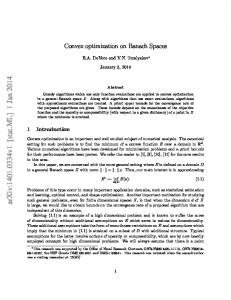
30

Fig. 1. The true state is marked by o, and the measured states by x. The dashed/solid line is the estimate from filter 3, respective 4. estimate of the state vector, without any problems with local minima. Compared to the Kalman filter, the advantage is that any log-concave noise distribution can be used and any linear equality or convex inequality state contraint may be included, while the main drawback is that no recursive convex optimization algorithm is yet available, which makes the approach computer intensive.

3. The convex optimization filter with constraint (20). 9. REFERENCES

4. The optimal filter (16). The numerical example is taken from [9], where   0.9 0.1 A=C= 0.1 0.9

[1] D.G. Robertson and J.H. Lee, “On the use of constraints in least squares estimation and control,” Automatica, vol. 38, pp. 1113–1123, 2002.

(21)

In Table 2, the root mean square error (RMSE) is given for these four cases and in Fig. 1 the states are shown. From 1. 2. 3. 4.

Kalman filter 6.1 with x1 + x2 = 1 6.1 with x1 + x2 = 1 and x ≥ 0 Optimal filter

0.585 0.573 0.566 0.403

Table 2. RMSE values for the different filters. this table it is obvious that we can obtain better estimates by using more information in this case. Of course, the convex optimization filters cannot compare to the performance of the optimal filter. However, the point is to show the flexibility of the approach, and the problem of consideration can be generalized with more contraints or a more complicated measurement relation, such that the optimal filter does no longer exist. 8. CONCLUSIONS We have formulated the state estimation problem in a convex optimization framework. In this way, well-known numerical efficient algorithms can be used to compute the MAP

[2] L. Vandenberghe and S. Boyd, “Convex optimization,” To be published, December 2001. [3] A.H. Jazwinski, Stochastic processes and filtering theory, Mathematics in science and engineering. Academic press, New York, 1970. [4] D.G. Luenberger, “Dynamic equations in descriptor form,” IEEE Transactions on Automatic Control, vol. AC-22, no. 3, jun 1977. [5] H.W. Sorenson, “Least-squares estimation: from gauss to kalman,” IEEE Spectrum, vol. 7, pp. 63–68, July 1970. [6] T. Kailath, “A view of three decades of linear filtering theory,” IEEE Transactions on Information Theory, vol. IT-20, no. 2, pp. 146–181, March 1974. [7] C.V. Rao, Moving Horizon Strategies for the Constrained Monitoring and Control of Nonlinear Discrete-Time Systems, Ph.D. thesis, University of Wisconsin Madison, 2000. [8] T. Kailath, A.H. Sayed, and B. Hassibi, Linear Estimation, Information and System Sciences Series. Prentice Hall, Upper Saddle River, New Jersey, 2000. [9] S. Andersson, Hidden Markov Models - Traffic Modeling and Subspace Methods, Ph.D. thesis, Centrum for Mathematical Sciences, Mathematical Statistics, Lund University, Lund, Sweden, 2002.