Convex Optimization. Pieter Abbeel. UC Berkeley EECS. Many slides and figures
adapted from Stephen Boyd. [optional] Boyd and Vandenberghe, Convex ...
Bellman’s curse of dimensionality n n
n
n-dimensional state space Number of states grows exponentially in n (assuming some fixed number of discretization levels per coordinate) In practice n
Discretization is considered only computationally feasible up to 5 or 6 dimensional state spaces even when using n n
Variable resolution discretization Highly optimized implementations
Optimization for Optimal Control n
n
n
n
Goal: find a sequence of control inputs (and corresponding sequence of states) that solves:
Generally hard to do. In this set of slides we will consider convex problems, which means g is convex, the sets Ut and Xt are convex, and f is linear. Next set of slides will relax these assumptions. Note: iteratively applying LQR is one way to solve this problem if there were no constraints on the control inputs and state. In principle (though not in our examples), u could be parameters of a control policy rather than the raw control inputs.
Convex Optimization Pieter Abbeel UC Berkeley EECS
Many slides and figures adapted from Stephen Boyd [optional] Boyd and Vandenberghe, Convex Optimization, Chapters 9 – 11 [optional] Betts, Practical Methods for Optimal Control Using Nonlinear Programming
Outline n
Convex optimization problems
n
Unconstrained minimization n
Gradient Descent
n
Newton’s Method
n
Equality constrained minimization
n
Inequality and equality constrained minimization
Convex Functions n
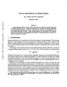
A function is f: 0, -(1/t) log(-u) is a smooth approximation of I_(u)
approximation improves for t à 1, better conditioned for smaller t
Equality and Inequality Constrained Minimization
Barrier Method n
Given: strictly feasible x, t=t(0) > 0, µ > 1, tolerance ² > 0
n
Repeat 1.
Centering Step. Compute x*(t) by solving
starting from x 2.
Update. x := x*(t).
3.
Stopping Criterion. Quit if m/t < ²
4.
Increase t. t := µ t
Example 1: Inequality Form LP
Example 2: Geometric Program
Example 3: Standard LPs
Initalization n
Basic phase I method: Initialize by first solving:
n
n
Easy to initialize above problem, pick some x such that Ax = b, and then simply set s = maxi fi(x) Can stop early---whenever s < 0
Initalization n
Sum of infeasibilities phase I method:
n
Initialize by first solving:
n
n
Easy to initialize above problem, pick some x such that Ax = b, and then simply set si = max(0, fi(x)) For infeasible problems, produces a solution that satisfies many more inequalities than basic phase I method
Other methods n
We have covered a primal interior point method n
n
one of several optimization approaches
Examples of others: n
Primal-dual interior point methods
n
Primal-dual infeasible interior point methods
Optimal Control (Open Loop) n
For convex gt and fi, we can now solve:
Which gives an open-loop sequence of controls
Optimal Control (Closed Loop) n
Given:
n
For k=0, 1, 2, …, T n
Solve min x,u
s.t.
T �
gt (xt , ut )
t=k
xt+1 = At xt + Bt ut fi (x, u) ≤ 0, xk = x ¯k
à à
∀t ∈ {k, k + 1, . . . , T − 1}
∀i ∈ {1, . . . , m}
n
Execute uk
n
Observe resulting state,
= an instantiation of Model Predictive Control. Initialization with solution from iteration k-1 can make solver very fast (and would be done most conveniently with infeasible start Newton method)
CVX n
Disciplined convex programming n
= convex optimization problems of forms that it can easily verify to be convex
n
Convenient high-level expressions
n
Excellent for fast implementation
n
n
Designed by Michael Grant and Stephen Boyd, with input from Yinyu Ye. Current webpage: http://cvxr.com/cvx/
CVX n
Matlab Example for Optimal Control, see course webpage