6. 1.3.2 Example of Importance of a 3-axis Accelerometer . . . . . . . . . 10 ..... niques since they are very sensitive to muscle activation and thus provide ... of the new generation personal electronic devices such as Apple iPhone [11], Nintendo wii.
A Novel Accelerometer-based Gesture Recognition System
by
Ahmad Akl
A thesis submitted in conformity with the requirements for the degree of Master of Applied Science Graduate Department of Electrical and Computer Engineering University of Toronto
Copyright
© 2010 by Ahmad Akl
Abstract A Novel Accelerometer-based Gesture Recognition System Ahmad Akl Master of Applied Science Graduate Department of Electrical and Computer Engineering University of Toronto 2010 Gesture Recognition provides an efficient human-computer interaction for interactive and intelligent computing. In this work, we address the problem of gesture recognition using the theory of random projection and by formulating the recognition problem as an `1 -minimization problem. The gesture recognition uses a single 3-axis accelerometer for data acquisition and comprises two main stages: a training stage and a testing stage. For training, the system employs dynamic time warping as well as affinity propagation to create exemplars for each gesture while for testing, the system projects all candidate traces and also the unknown trace onto the same lower dimensional subspace for recognition. A dictionary of 18 gestures is defined and a database of over 3,700 traces is created from 7 subjects on which the system is tested and evaluated. Simulation results reveal a superior performance, in terms of accuracy and computational complexity, compared to other systems in the literature.
ii
Dedication To my sister Zeina
iii
Acknowledgements I would like to thank all the people who have helped and inspired me during the pursuit of my masters degree. First, I would like to thank my supervisor, Prof. Shahrokh Valaee, for his guidance during my research and study at the University of Toronto. Prof. Valaee was always accessible and willing to help with my research making my research experience a smooth and a rewarding one. I also would like to thank all my lab mates at Wirlab (Wireless and Internet Research Laboratory) for making the lab a friendly place to work. I, especially, would like to thank Veria Nassab and Le Zhang for their incredible help and assistance. If it were not for them, I don’t think that I would have been able to make it through. My deepest gratitude and appreciation to my family for their unyielding love and support throughout my life; this thesis would have simply been impossible without their help. I am completely indebted to my father, for his overwhelming care and encouragement. Being the person he is, he strived all along to support the family and spared no effort to provide the best life for me. As for my mother, I could not have asked for more from her. No words can express my appreciation to her for her everlasting love and her constant support whenever I encountered difficulties. Finally, I cannot leave out my sister and brothers who have always been there for me with their prayers and advice. My sincere appreciation to my wife Rebecca whose dedication, love, and persistent confidence in me, have constantly taken the load off my shoulders. The past two years would not have been the same without her. Above all, thanks be to God for all the blessings in my life and for giving me this opportunity to achieve a higher level of education. My life has become more bountiful.
iv
Contents 1 Introduction
1
1.1
Motivation . . . . . . . . . . . . . . . . . . . . . . . . . . . . . . . . . . .
1
1.2
Gestures and Gesture Recognition . . . . . . . . . . . . . . . . . . . . . .
2
1.3
Means of Acquisition . . . . . . . . . . . . . . . . . . . . . . . . . . . . .
4
1.3.1
Wiimote(Wii Remote) . . . . . . . . . . . . . . . . . . . . . . . .
6
1.3.2
Example of Importance of a 3-axis Accelerometer . . . . . . . . .
10
1.4
Scope and Objectives . . . . . . . . . . . . . . . . . . . . . . . . . . . . .
13
1.5
Methodology . . . . . . . . . . . . . . . . . . . . . . . . . . . . . . . . .
14
1.6
Contributions . . . . . . . . . . . . . . . . . . . . . . . . . . . . . . . . .
15
2 Background 2.1
2.2
2.3
2.4
18
Dynamic Time Warping . . . . . . . . . . . . . . . . . . . . . . . . . . .
18
2.1.1
Example of Dynamic Time Warping . . . . . . . . . . . . . . . . .
21
Affinity Propagation . . . . . . . . . . . . . . . . . . . . . . . . . . . . .
22
2.2.1
Similarity Function . . . . . . . . . . . . . . . . . . . . . . . . . .
22
2.2.2
Message Passing: Responsibility and Availability . . . . . . . . .
23
2.2.3
Cluster Decisions . . . . . . . . . . . . . . . . . . . . . . . . . . .
24
Compressive Sensing . . . . . . . . . . . . . . . . . . . . . . . . . . . . .
25
2.3.1
Restricted Isometry Property (RIP) . . . . . . . . . . . . . . . . .
26
Random Projection . . . . . . . . . . . . . . . . . . . . . . . . . . . . . .
28
v
2.5
Hidden Markov Models . . . . . . . . . . . . . . . . . . . . . . . . . . . .
30
2.5.1
Three Basic Problems for HMMs . . . . . . . . . . . . . . . . . .
33
2.5.2
Solutions to the Three Basic Problems of HMMs . . . . . . . . . .
34
2.5.3
Types of HMMs . . . . . . . . . . . . . . . . . . . . . . . . . . . .
36
3 Gesture Recognition Systems
39
3.1
uWave . . . . . . . . . . . . . . . . . . . . . . . . . . . . . . . . . . . . .
39
3.2
System of Discrete HMMs . . . . . . . . . . . . . . . . . . . . . . . . . .
42
3.3
Proposed Gesture Recognition System . . . . . . . . . . . . . . . . . . .
43
3.3.1
Problem Setup . . . . . . . . . . . . . . . . . . . . . . . . . . . .
43
3.3.2
Training Stage
. . . . . . . . . . . . . . . . . . . . . . . . . . . .
45
3.3.3
Testing Stage . . . . . . . . . . . . . . . . . . . . . . . . . . . . .
48
4 Implementation Results
56
4.1
Distance Calculation System . . . . . . . . . . . . . . . . . . . . . . . . .
56
4.2
Gesture Recognition System . . . . . . . . . . . . . . . . . . . . . . . . .
57
5 Conclusions and Future Work 5.1
65
Future Work . . . . . . . . . . . . . . . . . . . . . . . . . . . . . . . . . .
Bibliography
67 68
vi
List of Tables 2.1
Computation of the similarity cost using DTW . . . . . . . . . . . . . . .
22
3.1
uWave Quantization Table . . . . . . . . . . . . . . . . . . . . . . . . . .
41
4.1
Performance of distance estimating system . . . . . . . . . . . . . . . . .
57
vii
List of Figures 1.1
A sideview, a topview, and a bottomview of the wiimote . . . . . . . . .
6
1.2
Wiimote with coordinate system labels . . . . . . . . . . . . . . . . . . .
7
1.3
Acceleration waveforms defining the gesture of moving the hand in a clockwise circle . . . . . . . . . . . . . . . . . . . . . . . . . . . . . . . . . . .
1.4
Acceleration waveforms defining the simple gesture of moving the hand to the right with the normal orientation of the wiimote
1.5
. . . . . . . . . . .
9
Acceleration waveforms defining the simple gesture of moving the hand to the right with a 90o clockwise rotation of the wiimote
1.6
8
. . . . . . . . . .
9
Acceleration waveforms defining the simple gesture of moving the hand to the right with the wiimote pointing up . . . . . . . . . . . . . . . . . . .
10
1.7
Acceleration waveforms for a person taking 10 steps . . . . . . . . . . . .
11
1.8
Equivalent acceleration waveform . . . . . . . . . . . . . . . . . . . . . .
12
2.1
Two time sequences P and Q that are similar but out of phase . . . . . .
19
2.2
Aligning the two sequences by finding the optimum warping path . . . .
21
2.3
A four-state ergodic HMM . . . . . . . . . . . . . . . . . . . . . . . . . .
36
2.4
A five-state left-right HMM . . . . . . . . . . . . . . . . . . . . . . . . .
37
3.1
Block diagram of the uWave System from [1] . . . . . . . . . . . . . . . .
40
3.2
Block diagram of the HMM-based System in [2] . . . . . . . . . . . . . .
42
3.3
General Overview of the Gesture Recognition System . . . . . . . . . . .
45
viii
3.4
Block Diagram of Training Stage . . . . . . . . . . . . . . . . . . . . . .
48
3.5
Block Diagram of Testing Stage . . . . . . . . . . . . . . . . . . . . . . .
49
4.1
The dictionary of 18 gestures . . . . . . . . . . . . . . . . . . . . . . . .
58
4.2
System’s performance against the number of gestures using a Gaussian random projection matrix compared to HMM . . . . . . . . . . . . . . .
4.3
System’s performance against the number of gestures using a sparse random projection matrix compared to HMM . . . . . . . . . . . . . . . . .
4.4
62
Comparison of testing computational cost between proposed system and system of HMMs . . . . . . . . . . . . . . . . . . . . . . . . . . . . . . .
4.6
61
Comparison of training computational cost between proposed system and system of HMMs . . . . . . . . . . . . . . . . . . . . . . . . . . . . . . .
4.5
60
62
Cdfs of the system’s performance for N = 8, 10, 16, and 18 gestures using a Gaussian random projection matrix . . . . . . . . . . . . . . . . . . . .
ix
63
Chapter 1 Introduction 1.1
Motivation
A variety of spontaneous gestures, such as finger, hand, body, or head movements are used to convey information in interactions among people. Gestures can hence be considered a natural communication channel with numerous aspects to be utilized in humancomputer interaction. Up to date, most of our interactions with computers are performed with traditional keyboards, mouses, and remote controls designed mainly for stationary interaction. With the help of the great technological advancement, gesture-based interfaces can serve as an alternate modality for controlling computers, e.g. to navigate in office applications or to play some console games like Nintendo Wii [3]. Gesture-based interfaces can enrich and diversify interaction options and provide easy means to interact with the surrounding environment especially for handicapped people who are unable to live their lives in a traditional way. On the other hand, mobile devices, such as PDAs, mobile phones, and other portable personal electronic devices provide new possibilities for interacting with various applications, if equipped with the necessary devices especially with the proliferation of low-cost MEMS (Micro-Electro-Mechanical Systems) technology. The majority of the new gen1
Chapter 1. Introduction
2
eration of smart phones, PDAs, and personal electronic devices are embedded with an accelerometer for various applications. Small wireless devices containing accelerometers could be integrated into clothing, wristwatches, or other personal electronic devices to provide a means for interacting with different environments. By defining some simple gestures, these devices could be used to control home appliances for example, or the simple up and down hand movement could be used to operate a garage door, or adjust the light intensity in a room or an office.
1.2
Gestures and Gesture Recognition
Expressive and meaningful body motions involving physical movements of the hands, arms, or face can be extremely useful for 1) conveying meaningful information, or 2) interacting with the environment. This involves: 1) a posture: a static configuration without the movement of the body part and 2) a gesture: a dynamic movement of the body part. Generally, there exist many-to-one mappings from concepts to gestures and vice versa. Hence gestures are ambiguous and incompletely specified. For example, the concept “stop” can be indicated as a raised hand with the palm facing forward, or an exaggerated waving of both hands over the head. Similar to speech and handwriting, gestures vary between individuals, and even for the same individual between different instances. Sometimes a gesture is also affected by the context of preceding as well as following gestures. Moreover, gestures are often language- and culture-specific. They can broadly be of the following types [4]: hand and arm gestures: recognition of hand poses, sign languages, and entertain-
ment applications (allowing children to play and interact in virtual environments). head and face gestures: Some examples are a) nodding or head shaking, b) direction
of eye gaze, c) raising the eyebrows, d) opening and closing the mouth, e) winking, f) flaring the nostrils, e) looks of surprise, happiness, disgust, fear, sadness, and
Chapter 1. Introduction
3
many others represent head and face gestures. body gestures: involvement of full body motion, as in a) tracking movements of two
people having a conversation, b) analyzing movements of a dancer against the music being played and the rhythm, c) recognizing human gaits for medical rehabilitation and athletic training. Gesture recognition refers to the process of understanding and classifying meaningful movements of the hands, arms, face, or sometimes head, however hand gestures are the most expressive, natural, intuitive and thus, most frequently used. Gesture recognition has become one of the hottest fields of research for its great significance in designing artificially intelligent human-computer interfaces for various applications which range from sign language through medical rehabilitation to virtual reality. More specifically, gesture recognition can be extremely useful for: Sign language recognition in order to develop aids for the hearing impaired. For
example, just as speech recognition can transcribe speech to text, some gestures representing symbols through sign language can be transcribed into text. Socially assistive robotics. By using proper sensors and devices, like accelerometers
and gyros, worn on the body of a patient and by reading the values from those sensors, robots can assist in patient rehabilitation. Developing alternative computer interfaces. Foregoing the traditional keyboard
and mouse setup to interact with a computer, gesture recognition can allow users to accomplish frequent or common tasks using hand gestures to a camera. Interactive game technology. Gestures can be used to control interactions within
video games providing players with an incredible sense of immersion in the totally engrossing environment of the game.
Chapter 1. Introduction
4
Remote Controlling. Through the use of gesture recognition, various hand gestures
can be used to control different devices, like secondary devices in a car, TV set, operating a garage door, and many others. Gesture recognition consists of gesture spotting that implies determining the start and the end points of a meaningful gesture trace from a continuous stream of input signals, and, subsequently, segmenting the relevant gesture. This task is very difficult due to two main reasons. First of all, the segmentation ambiguity in the sense that as the hand motion switches from one gesture to another, there occur intermediate movements as well. These transition motions are also likely to be segmented and matched with template traces, and need to be eliminated by the model. The spatio-temporal variability is the second reason since the same gesture may vary dynamically in duration and, very possibly in shape even for the same gesturer.
1.3
Means of Acquisition
The first step in recognizing gestures is sensing the human body position, configuration (angles and rotations), and movement (velocities or accelerations). This can be done either by using sensing devices attached to the user which can take the form of magnetic field-trackers, instrumental (colored) gloves, and body suits or by using cameras and computer vision techniques [4]. Each sensing technology varies along several dimensions, including accuracy, resolution, latency, range of motion, user comfort, and cost. Glovebased gestural interfaces typically require the user to wear a cumbersome device and carry a load of cables connecting the device to the computer. This hinders the ease and naturalness of the user’s interaction with the computer. Vision-based techniques, while overcoming this problem, need to contend with other problems related to occlusion of parts of the user’s body. Most of the work on gesture recognition available in the literature is based on computer vision techniques [5] [6] [7] [8] [9]. Vision-based techniques
Chapter 1. Introduction
5
vary among themselves in 1) the number of cameras used, 2) their speed and latency, 3) the structure of environment such as lighting and speed of movement, 4) any user requirements such as any restrictions on clothing, 5) the low-level features used such as edges, regions, silhouettes, moments, histograms, and others, and 6) whether 2D or 3D is used [4]. Therefore, these limitations restrict the applications of vision-based systems in smart environments. More specifically, suppose you are enjoying watching movies in your home theatre with all the lights off. If you decide to change the volume of the TV with a gesture, it turns out to be rather difficult to recognize your gesture under poor lighting conditions using a vision-based system. Furthermore, it would be extremely uncomfortable and unnatural if you have to be directly facing the camera to complete a gesture. A very promising alternative is to resort to other sensing techniques such as accelerationbased techniques or electromyogram-based (EMG-based) techniques. Acceleration-based gesture control is well-suited to distinguish noticeable, larger scale gestures with different hand trajectories. However, it is not very effective when it comes to detecting more subtle finger movements which is completely overcome by electromyogram-based techniques since they are very sensitive to muscle activation and thus provide rich information about finger movements. Yet, due to some inherent problems with EMG measurements including separability and reproducibility of measurements, the size of discriminable hand gesture set is limited to 4-8 gestures [10]. As a result, in this thesis and after examining all the sensing devices and techniques in literature, a 3-axis accelerometer is the sensing device utilized to acquire the data pertaining to gestures. Gesture recognition based on data from an accelerometer is an emerging technique for gesture-based interaction after the rapid development of the MEMS technology. Accelerometers are embedded in most of the new generation personal electronic devices such as Apple iPhone [11], Nintendo wii mote [12] which provide new possibilities for interaction in a wide range of applications, such as home appliances, in offices, and in video games. In the sequel, we represent
Chapter 1. Introduction
6
Figure 1.1: A sideview, a topview, and a bottomview of the wiimote vectors by bold lower case letters, e.g. r, matrices by bold upper case letters, e.g. R, and sets by calligraphic upper case letters, R.
1.3.1
Wiimote(Wii Remote)
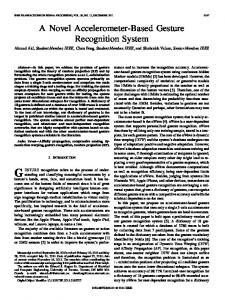
The wiimote, short for Wii Remote, is the primary controller for Nintendo Wii console [3]. Fig. 1.1 shows a sideview, a topview, and a bottomview of the wiimote. The wiimote provides an inexpensive and robust packaging of several useful sensors, with the ability to rapidly relay the information to the computer [12]. The Wiimote connects to a computer wirelessly through Bluetooth technology. When both the 1 and 2 buttons are pressed simultaneously, the Wiimote’s LEDs blink, indicating it is in discovery mode. A main feature of the wiimote is its motion sensing capability, which allows the user to interact with and manipulate items on screen via gesture recognition and the use of a 3-axis linear accelerometer and optical sensor technology. The accelerometer is physically rated to measure accelerations over a range of at least ±3g with 10% sensitivity [13] and reports acceleration in the device’s x-, y-, and z-directions, expressed in the unit of gravity g.
7
Chapter 1. Introduction
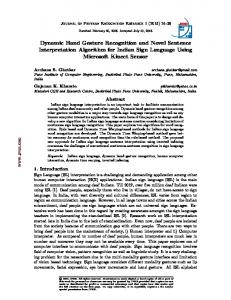
Figure 1.2: Wiimote with coordinate system labels 0
This reported acceleration vector is composed of the wiimote’s actual acceleration a and the Earth’s gravity ag , so obtaining the actual acceleration of the movement requires 0
subtracting the gravity vector from the wiimote’s reported acceleration, i.e. a = a − ag .
Due to its ease of use and familiarity in the world of human-computer interaction, the wiimote is chosen in this thesis as the device to acquire the different gesture traces and to relay the information to the computer. Accordingly, it is worth briefly describing how the remote works and how exactly it senses the change in acceleration. Fig. 1.2 shows a picture of the wiimote with labels to indicate the wiimote’s coordinate system and to show how the acceleration changes in the shown directions [14]. For example, if you are holding the wiimote naturally, i.e. +z pointing up, and you move the wiimote towards the top right corner of the room you are in, then you would expect to observe a decrease in the x- and the y-accelerations and an increase in the z-acceleration. The embedded 3-axis accelerometer detects the changes in acceleration by measuring the force exerted by a set of small proof masses inside of it with respect to its enclosure,
8
Chapter 1. Introduction
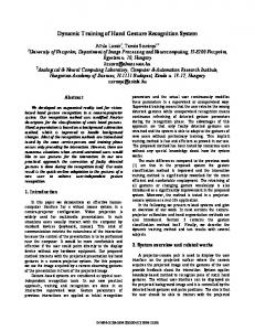
2 acceleration in x−direction acceleration in y−direction acceleration in z−direction
Acceleration (xg)
1.5 1 0.5 0 −0.5 −1 0
0.1
0.2
0.3
0.4 Time (sec)
0.5
0.6
0.7
Figure 1.3: Acceleration waveforms defining the gesture of moving the hand in a clockwise circle
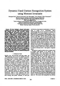
and therefore measures linear acceleration in a free fall frame of reference. In other words, if the Wiimote is in free fall, it will report zero acceleration. At rest and the normal orientation, it will report an upward acceleration in the positive z-direction equal to the acceleration due to gravity, g (approximately 9.8 m/s) but in the opposite direction. Fig. 1.3 shows the acceleration waveforms for moving the hand in a clockwise circle. The solid line represents the acceleration in the x-direction, the dashed line represents the acceleration in the y-direction, and the solid-dot line represents the acceleration in the z-direction. According to the way the accelerometer is manufactured, tilting the accelerometer can result in different measurements for the same hand movement. Fig. 1.4 shows the acceleration waveforms representing a simple hand movement to the right. The wiimote is held in a horizontal orientation as shown in Fig. 1.2. However, Fig. 1.5 shows the acceleration waveforms representing the same hand movement to the right but with the wiimote held up-side down. Notice how the constant acceleration of magnitude g is now in the negative z-direction. In this scenario, the waveforms in the x- and the ydirections are similar to a movement of the hand to the left. This can be a major source
9
Chapter 1. Introduction
2
normalised acceleration (m/s )
1.5
1
0.5
0
−0.5
−1 0
acceleration in x−direction acceleration in y−direction acceleration in z−direction 0.05
0.1
0.15
0.2
0.25
0.3
0.35
0.4
0.45
0.5
time (sec)
Figure 1.4: Acceleration waveforms defining the simple gesture of moving the hand to the right with the normal orientation of the wiimote
0.8 acceleration in x−direction acceleration in y−direction acceleration in z−direction
2
normalised acceleration (m/s )
0.6 0.4 0.2 0 −0.2 −0.4 −0.6 −0.8 −1 −1.2 0
0.1
0.2
0.3
0.4
0.5
0.6
time (sec)
Figure 1.5: Acceleration waveforms defining the simple gesture of moving the hand to the right with a 90o clockwise rotation of the wiimote
10
Chapter 1. Introduction
0.8
2
normalised acceleration (m/s )
0.6 0.4 0.2 0 acceleration in x−direction acceleration in y−direction acceleration in z−direction
−0.2 −0.4 −0.6 −0.8 −1 −1.2 0
0.1
0.2
0.3
0.4
0.5
0.6
time (sec)
Figure 1.6: Acceleration waveforms defining the simple gesture of moving the hand to the right with the wiimote pointing up of confusion. Yet, the acceleration in the z-direction can indicate that the wiimote is held up-side down. Fig. 1.6 shows the acceleration waveforms, again, representing the same hand movement to the right but with the wiimote pointing up in a vertical orientation. In this case, the constant acceleration of magnitude g is now in the negative y-direction. This highlights the fact that tilting the wiimote while performing a gesture can lead to different measurements. All the above waveforms address how serious the issue of tilting can be and how it should definitely be taken into account while designing a gesture recognition system with data acquired using a wiimote.
1.3.2
Example of Importance of a 3-axis Accelerometer
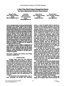
Again, the accelerometer is a device for measuring the acceleration of moving objects. Fig. 1.7 shows the raw acceleration waveforms acquired by a wiimote for a person walking a distance of 22 ft. Theoretically, the speed can be obtained by integrating the acceleration
11
Chapter 1. Introduction
1.4
2
normalised acceleration (m/s )
1.2 1 0.8
X−acceleration Y−acceleration Z−acceleration
0.6 0.4 0.2 0 −0.2 0
1
2
3
4 5 time (sec)
6
7
8
9
Figure 1.7: Acceleration waveforms for a person taking 10 steps
signals and further integrating the speed to obtain the distance. However, for indoor environments, the acceleration is very small and therefore it is very challenging to separate it from the noise due to the channel, offset drift, internal calibration, or even tilting. Consequently, integrating the acceleration results in integrating the error and leads to erroneous estimation of the distance. Alternatively, detecting the number of footsteps taken to walk a distance can help in knowing the distance covered if the stride size is known. In other words, the distance can be related to the number of steps and the step size as follows distance = stride size × number of steps
(1.1)
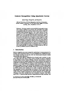
When walking with an accelerometer, the acceleration in the conventional z-direction fluctuates in a sinusoidal form as a result of the motion mechanism as shown in Fig. 1.7. Notice how clear the peaks are in the z-direction, and the acceleration waveforms in the x-, and y-directions seem to carry some useful information too. It turns out that adding the acceleration values in the three directions emphasizes the peaks and makes them more significant as is depicted in Fig. 1.8. Each significant peak represents one
12
Chapter 1. Introduction
sum of normalised accelerations (m/s2)
0.4 0.3 0.2 0.1 0 −0.1 −0.2 −0.3 0
1
2
3
4 5 time (sec)
6
7
8
9
Figure 1.8: Equivalent acceleration waveform step, and accordingly the subject walked 10 steps in order to cover the distance of 22 ft. To estimate the number of steps, a simple zero crossing algorithm is used since it is obvious that the acceleration waveform crosses the zero line twice for each step. As a result, the number of steps can be found by detecting the number of zero crossings and dividing it by 2. As for the stride size, it is found empirically using the relationship proposed in [15] and which states that
stride size =
p 4
Amax − Amin × K
(1.2)
where Amin is the minimum acceleration measured in the z-axis in a single stride. Amax is the maximum acceleration measured in the z-axis in a single stride. K is a constant for unit conversion, obtained by walking training
Some more accurate, but more complex models for calculating the number of steps and step size are available in the literature [16] [17]. A simple distance calculating system
Chapter 1. Introduction
13
using a single 3-axis accelerometer is developed and simulated in Section 4.1 of Chapter 4. Simulations show the accelerometers can be of great significance and open the door to numerous applications.
1.4
Scope and Objectives
The objective of this work is to create a novel system that can automatically recognize hand gestures using a single 3-axis accelerometer and that utilizes the sparse nature of the gesture sequence. The proposed system can be implemented for user-dependent recognition, mixed-user recognition, and user-independent recognition. User-dependent recognition refers to the process of training a system using data from a single subject and using the system specifically for this subject only. Mixed-user recognition is more general in the sense that more than one subject can be used to train the system under the condition that the same subjects are involved in using the system. Finally, userindependent recognition, as the name implies, refers to the process of recognizing the input signals independently of the user. In other words, use of the system is not restricted to those involved in training the system. The proposed system evolves to be greatly competitive against the statistical models and the other existing gesture recognition systems in terms of computational complexity and recognition accuracy. Chapter 2 presents the relevant background material. The details of how dynamic time warping and affinity propagation work are introduced. Then this chapter discusses random projection and how it can serve as an excellent approximation of signals with fewer samples. After that, the theory of Hidden Markov Models (HMMs) is presented followed by a literature review of previous systems that have been developed to recognize gestures using a single 3-axis accelerometer. Chapter 3 introduces the proposed gesture recognition system. The system utilizes dynamic time warping to overcome the problem of different durations of gesture traces
Chapter 1. Introduction
14
and to compute a cost of similarity between the different gesture traces. Affinity propagation is then implemented to train the system and to create an exemplar or a set of exemplars for each gesture. Finally, the candidate gesture traces are randomly projected onto the same lower subspace to recognize an unknown gesture trace. Chapter 4 presents a prototype implementation of the proposed system. The different parameters are defined to simulate the system. Results are presented and compared to other gesture recognition systems available in the literature that are based on a single 3-axis accelerometer. These include, continuous HMMs, uWave [1], and a system of discrete HMMs in [2]. Finally, in Chapter 5 we end this work with our concluding remarks and provide directions for future work.
1.5
Methodology
The first step in developing the gesture recognition system is to construct a dictionary of gestures on which the system will operate. So for a system of N gestures, we collect M traces for each gesture to create a database of the defined gestures. The database is then split into a training dataset and a testing dataset. Gesture data for the proposed system refers to the acceleration of the hand, measured at different times t using a single 3-axis accelerometer. However, hand gestures inherently suffer from temporal variations, and consequently, traces of the same gesture are of different lengths which poses the first major challenge in developing a gesture recognition system. In order to overcome this problem, dynamic time warping algorithm is used to compute a cost of similarity between the different gesture traces. Affinity propagation then operates on the costs of similarities to divide the training dataset into different clusters each represented by an “exemplar”. This similarity cost computation and clustering using affinity propagation represent the core of the training stage. Therefore, the
Chapter 1. Introduction
15
output of the training stage is a set of exemplars for the different gestures defined in the database. For testing, a user moves an accelerometer-equipped device to signal a particular gesture from the database. The objective of the gesture recognition system is to find out which gesture is intended by the user. To do that, the unknown trace is compared to the exemplars induced by affinity propagation to select a subset of coordinate traces. Based on the premise that the acquired gesture traces are sparse in nature, the candidate traces and the unknown gesture trace are projected onto the same lower-dimensional subspace in order to overcome the problem of different trace sizes. Projection is implemented using two definitions of a projection matrix: a matrix whose entities are independent realizations of Gaussian random variables and a matrix with sparse entities. Construction of random projection matrices is explained in full details in Section 2.4. Such definitions of the projection matrix are used since they satisfy the restricted isometry property (RIP) necessary for recovery of original data. After projection is done, the recognition problem is formulated as an `1 minimization problem whose solution gives the label of the unknown trace.
1.6
Contributions
The main contribution of this work is the design of a novel gesture recognition system based solely on data from a single 3-axis accelerometer. The proposed system is very efficient in terms of recognition accuracy and computational complexity and is very competitive with other systems in the literature. The following lists the contributions of this work, and any publications that refer to them: Single 3-axis Accelerometer : The system operates on data from only a single 3-
axis accelerometer. Most of the systems in the literature combine data from an
Chapter 1. Introduction
16
accelerometer with data from other sensing devices like EMG sensors, or gyroscopes in order to enhance the system’s performance. In addition, current systems that use only a single 3-axis accelerometer have limited applications, like being only userdependent as is the case with uWave system, or have a small dictionary size. On the other hand, our proposed system uses only a single 3-axis accelerometer and functions competitively for any kind of recognition, user-dependent, mixed-user, or user-independent. Furthermore, our dictionary size is the largest in published studies to the best of our knowledge. Dynamic Time Warping and Affinity Propagation: Our system uses dynamic time
warping to compute the cost of similarity between the different gesture traces followed by affinity propagation to split the training data into different clusters. Affinity propagation, being a very recent technique, has not been exploited in this field and according to the literature, it outperforms all the other clustering techniques. Besides, affinity propagation operates on a matrix of similarities between the gesture traces which makes it very suitable to the system set up (Chapter 2 and Chapter 3, [18], [19]). Random Projection: In the testing stage, comparing the unknown trace to the set
of exemplars, found in the training stage, using dynamic time warping only does not suffice. Yet, the problem of the different gesture traces still poses a problem and hinders any further processing. Therefore, random projection proves to be an efficient way of projecting all the candidate traces and at the same time, preserving the similarities and the differences between the traces (Chapter 2 and Chapter 3, [18], [19]). `1 Minimization Formulation : Formulating the recognition problem as an `1 min-
imization problem is based on the premise that the gesture traces are sparse in nature. So, after the candidate traces are projected, the recognition problem is
Chapter 1. Introduction
17
transformed into an `1 minimization problem and its solution leads to the classification of the unknown trace (Chapter 3, [18], [19]).
Chapter 2 Background 2.1
Dynamic Time Warping
The Euclidean distance is a very common metric used in many applications to represent the degree of similarity between any two sequences p = {p1 , . . . , pn } and q = {q1 , . . . , qn }. The cost of similarity based on the Euclidean distance metric is computed as v u n uX dEuclid(p, q) = t (pi − qi )2
(2.1)
i=1
This kind of metric is applicable when the two sequences p and q are of the same length. However, in case p and q are not of the same length then the Euclidean distance is not applicable as a similarity measure. Instead, a more flexible method that can find the best mapping from elements in p to those in q must be sought in order to find a similarity cost between two sequences of different lengths. Dynamic time warping (DTW) is an algorithm that measures the similarity between two time sequences of different durations. DTW matches two time signals by computing a temporal transformation causing the signals to be aligned. The alignment is optimal in the sense that a cumulative distance measure between the aligned samples is minimized 18
19
Chapter 2. Background
6 P Q
4
Magnitude
2 0 −2 −4 −6 −8 0
0.1
0.2
0.3
0.4 Time (sec)
0.5
0.6
0.7
0.8
Figure 2.1: Two time sequences P and Q that are similar but out of phase [20]. Assume that the two sequences, p and q, are similar but are out of phase and are of length n and m, respectively, where p = {p1 , . . . , pn } and q = {q1 , . . . , qm } as shown in Fig 2.1. The objective is to compute the matching cost: DTW(p, q). To align the two sequences using DTW, we construct an n × m matrix where the (i, j)-th entry of the matrix indicates the distance d(pi , qj ) between the two points pi and qj , where d(pi , qj ) = (pi − qj )2 . The cost of similarity between the two sequences is based on a warping path W that defines a mapping between p and q. The kth element of W is defined as wk which is a pointer to the k-th element on the path, usually represented by the indices of the corresponding element. So, W is defined as
W = hw1 , w2 , . . . , wk , . . . , wL i
(2.2)
max(m, n) ≤ L < n + m − 1
(2.3)
such that,
The warping path is subject to two main constraints [20]:
20
Chapter 2. Background
i. Boundary conditions: w1 = (1, 1) and wL = (n, m) and this entails that the warping path starts and ends in diagonally opposite corners of the matrix.
0
0
0
ii. Continuity and Monotocity: Given wk = (a, b), and wk−1 = (a , b ), then a ≤ a ≤ 0
0
0
a + 1 and b ≤ b ≤ b + 1. This casts a restriction on the allowable steps in the path to adjacent cells including diagonally adjacent cells, and forces the path’s indices to be monotonically increasing.
There are exponentially many warping paths that satisfy the above constraints. However, we are seeking only the path that minimizes the warping cost. In other words, v u L uX DTW(p, q) = min{t DTW(wk )}
(2.4)
k=1
The monotonically increasing warping path that minimizes the similarity cost between p and q is found by applying the dynamic programming formulation below, which defines the cumulative cost Di,j as the cost d(pi , qj ) in the current cell plus the minimum of the cumulative cost of the adjacent elements,
Di,j = d(pi , qj ) + min {Di,j−1, Di−1,j , Di−1,j−1}
(2.5)
DTW(p, q) = Dn,m
(2.6)
and consequently,
The resulting new matrix is depicted in Fig. 2.2 showing the optimum warping path between the two sequences and demonstrating the constraints that the warping path is satisfying.
21
Chapter 2. Background
P
Q
Figure 2.2: Aligning the two sequences by finding the optimum warping path
2.1.1
Example of Dynamic Time Warping
An example of how to use DTW to compute the similarity cost between two sequences p and q of different lengths is given here. Let
p = [1 2 2 3 3 4 4] q = [1 2 3 4] where q is a compressed version of p. In this case, n = 7 and m = 4 and we start by constructing a matrix which is 7 × 4 and placing p and q on each side of the matrix. The (i, j)-th element of the matrix consists of the d(pi , qj ) = (pi − qj )2 as shown in the table to the left below. After the matrix to the left is filled, a second matrix based on it is constructed where each (i, j)-th element of the second matrix represents the cost in the current cell of the matrix to the left plus the minimum cost from the adjacent cells in the matrix to the right as per the formulation in( 2.5). The cost between the two sequences p and q is equal to the cost in the top right corner of the second matrix which is 0 in this example.
22
Chapter 2. Background 4 4 3 3 2 2 1
9 9 4 4 1 1 0 1
4 4 1 1 0 0 1 2
1 1 0 0 1 1 4 3
0 0 1 1 4 4 9 4
→
28 19 10 6 2 1 0
10 6 2 1 0 0 1
2 1 0 0 1 1 5
0 0 1 1 5 5 14
Table 2.1: Computation of the similarity cost using DTW
2.2
Affinity Propagation
Clustering data based on a measure of similarity is a critical step in engineering systems. A common approach is to use data to learn a set of centers such that the sum of squared errors between data points and their nearest centers is small. When the centers are selected from actual data points, they are called exemplars. A new technique for data clustering is the Affinity Propagation (AP) algorithm [21]. AP is an algorithm that simultaneously considers all data points as potential exemplars and recursively transmits real-valued messages until a good set of exemplars and clusters emerges. An exemplar is a term used to represent the center selected from the the actual data points. AP does not require that the number of clusters be known prior to clustering, instead, the clusters emerge naturally.
2.2.1
Similarity Function
AP algorithm takes an input function of similarities, s(i, j), where s(i, j) reflects how well suited data point j is to be the exemplar of data point i. AP aims to maximize the similarity s(i, j) for every data point i and its chosen exemplar j. For example, the similarity function could be the negative Euclidean distance between data points. Negative Euclidean distance is used so that a maximum similarity corresponds to the closest data points. In addition to the measure of similarity, AP takes as input a set of real numbers,
23
Chapter 2. Background
known as self-similarity s(i, i), or preference (p) for each data point. The preference (p) influences the number of exemplars that are identified. Initializing a data point with a larger or smaller self-similarity, respectively increases or decreases the likelihood of the data point becoming an exemplar. If all the data points are initialized with the same constant self-similarity, then all data points are equally likely to become exemplars. The preference (p) also controls how many clusters are produced. By increasing and decreasing this common self-similarity input, the number of clusters produced is increased and decreased respectively. If all data points are assigned the median of the input similarities, a moderate number of clusters is produced, and if they are assigned the minimum of the input similarities, the smallest number of clusters is produced. This algorithm can generate better clusters, compared to other clustering techniques like K-means clustering, because of its initialization-independent property [21].
2.2.2
Message Passing: Responsibility and Availability
Clustering is based on the exchange of two types of messages: the “responsibility” message to decide which data points are exemplars and the “availability” message, to decide which cluster a data point belongs to: the responsibility message r(i, j) sent from data point i to candidate exemplar j,
reflects the accumulated evidence for how well-suited data point j is to serve as the 0
exemplar for i, taking into account other potential exemplars j for data point i, that is r(i, j) = s(i, j) − 0 max 0
j s.t.j 6=j
n o 0 0 a(i, j ) + s(i, j )
(2.7)
where i 6= j, and s(i, j) is the similarity between data point i and data point j and a(i, j) is the availability message defined below. the availability message a(i, j), sent from candidate exemplar j to data point i,
reflects the accumulated evidence for how appropriate it would be for data point i
24
Chapter 2. Background
to choose j as its exemplar, taking into account the support from other data points that j should be an exemplar, that is
a(i, j) = min
0, r(j, j) +
0
X
0
max{0, r(i , j)}
(2.8)
0
i s.t.i 6=i,j
The self-responsibility, r(j, j) and self-availability, a(j, j) are two additional mes-
sages calculated for each data point, j. Both of these messages reflect accumulated evidence that j is an exemplar, and they are used to find the clusters. The self-responsibility bases exemplar suitability on input preference and the maximum availability received from surrounding data points whereas the self-availability bases exemplar suitability on the number and strength of positive received responsibilities. Mathematically,
r(j, j) = s(j, j) − 0 max0
j s.t.j 6=i
a(j, j) = 0
X
n
0
0
a(j, j ) + s(j, j )
0
max{0, r(i , j)}
o
(2.9)
(2.10)
0
i s.t.i 6=j
2.2.3
Cluster Decisions
In AP algorithm, the exemplar of each data point i is found using the following equation,
exemplari = arg max{a(i, j) + r(i, j)} j
(2.11)
This clustering procedure may be performed at any iteration of the algorithm, but final clustering decisions should be made once the algorithm stabilizes. The algorithm can be terminated once exemplar decisions become constant for some number of iterations, indicating that the algorithm has converged. It should be noted that the algorithm possesses another useful feature: it is possible to determine when a specific data point
25
Chapter 2. Background
has converged to exemplar status for a specific iteration. When a data point’s selfresponsibility plus self-availability becomes positive, that data point has become the exemplar for its cluster.
2.3
Compressive Sensing
Compressive sensing [22] is a method that allows us to recover signals from far fewer measurements than the traditional sampling methods. Assume that the received signal can be represented as a d × 1 vector x = Ψs where Ψ is a d × d basis matrix and s is a d × 1 sparse vector that has only ls � d non-zero elements. The locations of the non-zero elements in s are unknown. Signal x is compressed using a k × d sensing matrix Φ, which yields the measurement vector y of dimension k as follows
y = Φx = ΦΨs
(2.12)
It has been shown that s can be recovered exactly if k satisfies the following inequality
k ≥ cls log (d/ls )
(2.13)
where c is a constant and ls is the sparsity level [22]. The signal can be reconstructed by solving the following `1 norm minimization problem
min ksk1 s
subject to y = ΦΨs
(2.14)
26
Chapter 2. Background
2.3.1
Restricted Isometry Property (RIP)
To explain the concept of Restricted Isometry Property (RIP), we refer to the approach outlined in [23] by describing the concept of compressive sensing in terms of encoder/decoder and approximation error. In the discrete compressive sensing problem, we are interested in economically recording the information about a vector or a signal x ∈ Rd . We allocate a budget of k nonadaptive questions to ask about x. Each question takes the form of a linear functional applied to x. Thus, the information we extract from x is given by y = Φx,
(2.15)
where Φ is a k × d matrix and y ∈ Rk . The matrix Φ maps Rd into Rk , where d � k. To extract the information that y holds about x, we use a decoder ∆ that maps from ¯ := ∆(y) = ∆(Φx) to Rk back into Rd . The role of ∆ is to provide an approximation x x. The mapping ∆ is typically nonlinear. The central question of compressive sensing is: What are the good encoder-decoder pairs (Φ, ∆)? To measure the performance of an encoder-decoder pair (Φ, ∆), we introduce a norm k · kX in which we measure error. Then, E(x, Φ, ∆)X :=k x − ∆(Φx) kX
(2.16)
is the error of the encoder-decoder on x. More generally, if K is any closed and bounded set contained in Rd , then the error of this encoder-decoder on K is given by E(K, Φ, ∆)X = sup E(x, Φ, ∆)X .
(2.17)
x∈K
Thus, the error on the set K is determined by the largest error on K. To address the question of what constitutes good encoder-decoder pairs, we introduce Ak,d := {(Φ, ∆) :
27
Chapter 2. Background Φ is k × d}. The best possible performance of an encoder-decoder on K is given by Ek,d (K)X :=
inf
(Φ,∆)∈Ak,d
E(K, Φ, ∆)X .
(2.18)
This is the so-called “minimax” way of measuring optimality that is prevalent in approximation theory, information-based complexity, and statistics [23]. The decoder ∆ is important in practical applications in compressive sensing and also in the above formulation. Cand`es, Romberg, and Tao [24] showed that decoding can be accomplished by the linear program
∆(y) := arg min k x k`d1 .
(2.19)
x:Φx=y
Furthermore, Cand`es and Tao [25] introduced the isometry condition on matrices Φ and established its important role in compressive sensing. Given a matrix Φ and any set T of column indices with the number of elements nT , we denote by ΦT the k × nT matrix composed of these columns. Similarly, for a vector x ∈ Rd , we denote by xT the vector obtained by retaining only the entries in x corresponding to the column indices T . We say that Φ satisfies the Restricted Isometry Property (RIP) of order m if there exists a δm ∈ (0, 1) such that (1 − δm ) k xT k2`d ≤k ΦT xT k2`k ≤ (1 + δm ) k xT k2`d 2
2
2
(2.20)
holds for all sets T with nT ≤ m. The condition (2.20) is equivalent to requiring that the Grammian matrix ΦTT ΦT has all of its eigenvalues in [1 − δm , 1 + δm ], where ΦTT denotes the transpose of ΦT . The “good” matrices for compressive sensing should satisfy (2.20) for the largest possible m. For example, Cand`es and Tao [25] show that whenever Φ satisfies the RIP
28
Chapter 2. Background of order 3m with δ3m < 1, then
k x − ∆(Φx) k`d2 ≤
C2 σm (x)`d1 √ , m
(2.21)
where σm (x)`d1 denotes the `1 error of the best m-term approximation, and the constant C2 depends only on δ3m . The original proof of (2.21) is given in [26] and the proof for this particular formulation is provided in [27]. The question before us now is how we can construct matrices Φ that satisfy the RIP for the largest possible range of m. The most prominent matrices are the k × d random matrices Φ whose entries φi,j are independent realizations of Gaussian random variables [23] 1 φi,j ∼ N (0, ). n
(2.22)
One can also use matrices where the entries are independent realizations of ±1 Bernoulli random variables [28]
φi,j =
+1 √ n
with probability
1 , 2
−1 √ n
with probability
1 , 2
(2.23)
or related distributions such as
φi,j
2.4
q + n3 with probability = 0 with probability q − 3 with probability n
1 , 6 2 , 3
(2.24)
1 . 6
Random Projection
Random Projection (RP) has recently emerged as a powerful technique for dimensionality reduction [29] [30]. In RP, the original d-dimensional data is projected onto a k-dimensional (k � d) subspace using a k × d random matrix A whose columns have
29
Chapter 2. Background
unit lengths. Using matrix notation, let Xd×n be the original set of n d-dimensional observations, then the projection problem can be formulated as, XRP k×n = Ak×d Xd×n
(2.25)
where XRP k×n represents the projected data onto the lower k-dimensional subspace.The concept of RP is inspired by the Johnson-Lindenstrauss theorem [31]. Strictly speaking, (2.25) is not a projection because the projection matrix A is generally not orthogonal and such a linear mapping can result in significant distortion to the original data set. One solution is to orthogonalize A but this can be computationally very expensive. Alternatively, we can resort to the fact that in a high-dimensional space, the number of almost orthogonal directions is much larger than the number of orthogonal directions [32]. Therefore, vectors having random directions can be sufficiently close to orthogonal and thus can offer the necessary preservation of the original data set after projection. In case of RP, the matrix A is the general case of Φ in Sections 2.3 and 2.3.1. A is a sampling operator for X, and is invertible if each x ∈ X is uniquely determined by its sampled or projected data Ax; this means if for every u, v ∈ X, Au = Av then u = v. In other words, A is a one-to-one mapping between XRP and X and this allows a unique identification for each x ∈ X from Ax. However, practically, we want that a small change in x only result in a small change in its sampled or projected data Ax. Therefore, we consider a stricter condition given by
α k u − v k2H ≤ k Au − Av k2l2 = ≤ β ku−v
k2H
X n
|hu − v, ψn2 i|2 (2.26)
where α and β are constants with α > 0 and β < ∞, H is an ambient Hilbert space, and ψn ∈ H is a sampling vector [33].
30
Chapter 2. Background
The sampling condition (2.26) on A is related to the important concept of restricted isometry property (RIP) described in Section 2.3.1, and is interestingly the same as RIP if X has sparse columns and the columns come from the same subspace [33] [34]. As mentioned in Section 2.3.1, any distribution of zero mean and unit variance satisfies the sampling condition in (2.26). As far as this thesis is concerned, Gaussian distributions as well as a special case of the distribution in (2.24) given below +1 with probability √ aij = 3 · 0 with probability −1 with probability
1 6 2 3
(2.27)
1 6
will be investigated. The distribution (2.27) has been reported to result in further computational savings since computations can be done using integer arithmetics [28].
2.5
Hidden Markov Models
Consider a system which may be described at any time as being in one of a set of N distinct states, S1 , S2 , . . ., SN . At regularly spaced discrete times, the system undergoes a change of state according to a set of probabilities associated with the state. We denote the time instants associated with the sate changes as t = 1, 2, . . . , and we denote the actual state at time t as qt . Generally, a full probabilistic description of such a system would require specification of the current state (at time t), as well as all the predecessor states. However, a system is first-order Markov if the conditional probability density of the current state qt , given all present and past states, depends only on the most recent state, represented in the following formulation:
P [qt = Sj |qt−1 = Si , qt−2 = Sk , · · · ] = P [qt = Sj |qt−1 = Si ].
(2.28)
31
Chapter 2. Background
Furthermore, we only consider those systems in which the right-hand side of (2.28) is independent of time, thereby leading to the set of state transition probabilities aij of the form aij = P [qt = Sj |qt−1 = Si ], 1 ≤ i, j ≤ N
(2.29)
with the state transition coefficients having the properties aij ≥ 0 PN j=1 aij = 1
(2.30)
A Hidden Markov Model (HMM) is a double stochastic process governed by 1) an underlying Markov chain with a finite number of states, and 2) a set of random functions associated with each state. HMM has proven to be extremely efficient in modeling timeseries with spatial and temporal variability as well as handling undefined patterns. The states in an HMM are connected by transitions. Each transition is associated with a pair of probabilities: (i) transition probability, the probability of transitioning from the current state to a different state, and (ii) output probability, the probability of producing an output symbol from a finite alphabet given a state. An HMM is formally characterized by the following [35]: i. N, the number of states in the model. Although the states are hidden, there is frequently some physical significance associated with the states or the sets of states in the model. States can be interconnected in different ways. Ergodic model interconnection is the simplest of all, and it represents the interconnection in which any states can be reached from any other state. The individual states are denoted as S = {s1 , s2 , s3 , . . . , sN }, and the state at time t is denoted by the random variable qt . ii. M, the number of distinct observation symbols per state, i.e. the discrete alphabet
32
Chapter 2. Background
size. The observation symbols, in other words, model the physical output of the system. The individual symbols are denoted as V = {v1 , v2 , v3 , . . . , vM }, and the observation at time t is denoted by the random variable Ot . iii. The state transition probability distribution A = {aij } where aij = P (qt+1 = Sj |qt = Si ), 1 ≤ i, j ≤ N
(2.31)
For the special case where any state can reach any other state in a single step, we have aij > 0 for all i,j. For other types of HMMs, aij = 0 for one or more (i, j) pairs. iv. The observation symbol probability distribution in state j, B = {bj (k)}, where bj (k) = P (vk at t|qt = Sj ), 1 ≤ j ≤ N
(2.32)
1≤k≤M v. The initial state distribution π = πi where
πi = P (q1 = Si ) 1 ≤ i ≤ N
(2.33)
Given appropriate values of N, M, A, B, and π, the HMM can be used as a generator to give an observation sequence
O = O1 O2 · · · OT
(2.34)
where each observation Ot is one of the symbols from V , and T is the number of observations in the sequence. The sequence O is generated as follows 1. Choose an initial state q1 = Si according to the initial state distribution π.
33
Chapter 2. Background 2. Set t = 1.
3. Choose Ot = vk according to the symbol probability distribution in state Si , i.e. bi (k). 4. Transit to a new state qt+1 = Sj according to the state transition probability distribution for state Si , i.e. aij . 5. Set t = t + 1; return to step 3 if t < T , otherwise terminate the procedure. For convenience, an HMM is represented in a compact form as
λ = (A, B, π)
(2.35)
to indicate the complete parameter set of the model.
2.5.1
Three Basic Problems for HMMs
Given the form of the HMM, there are three basic problems of interest that must be solved for the model to be useful in real-world applications [35]. These problems are the following: Problem 1 : Given the observation sequence O = O1 O2 · · · OT , and a model λ = (A, B, π), how do we efficiently compute P (O|λ), the probability of the observation sequence, given the model? Problem 2 : Given the observation sequence O = O1 O2 · · · OT , and the model λ, how do we choose a corresponding state sequence Q = q1 q2 · · · qT which is optimal is some meaningful sense? Problem 3 : How do we adjust the model parameter λ = (A, B, π) to maximize P (O|λ)?
34
Chapter 2. Background
2.5.2
Solutions to the Three Basic Problems of HMMs
As far as this thesis is concerned, we are interested only in solving Problems 1 and 3. Problem 1 is an evaluation problem, namely given a model and a sequence of observations, how do we compute the probability that the observed sequence was produced by the model. We can also view the problem as one of scoring how well a given model matches a given observation sequence. The latter concept is extremely useful, especially in the case when we are trying to choose among several competing models. The solution to Problem 1 allows us to choose the model which best matches the observations. As for Problem 3, it is a one in which we attempt to optimize the model parameters so as to best describe how a given observation sequence comes about. The observation sequence used to adjust the model parameters is called a training sequence since it is used to train the HMM.
A. Solution to Problem 1 In Problem 1, we wish to calculate the probability of the observation sequence, O = O1 O2 · · · OT , given the model λ, i.e. P (O|λ). The most straightforward way of doing this is through enumerating every possible state sequence of length T . Considering one such fixed state sequence
Q = q1 q2 · · · qT
(2.36)
where q1 is the initial state. The probability of the observation sequence O for the state sequence of (2.36) is
P (O|Q, λ) =
T Y t=1
P (Ot |qt , λ)
(2.37)
where we have assumed statistical independence of observations. Thus we get
P (O|Q, λ) = bq1 (O1 ) · bq2 (O2 ) · · · bqT (OT )
(2.38)
35
Chapter 2. Background The probability of such a state sequence Q can be written as
P (Q|λ) = πq1 aq1 q2 aq2 q3 · · · aqT −1 qT
(2.39)
The joint probability of O and Q, i.e. the probability that O and Q occur simultaneously, is simply the product of (2.38) and (2.39),
P (O, Q|λ) = P (O|Q, λ)P (Q, λ).
(2.40)
The probability of O given the model is obtained by summing the joint probability over all possible state sequences q giving
P (O|λ) =
X
P (O|Q, λ)P (Q|λ)
allQ
=
X
q1 ,q2 ,··· ,qT
πq1 bq1 (O1 )aq1 q2 bq2 (O2 ) · · · aqT −1 qT bqT (OT )
(2.41)
Calculating P (O|λ) according to this direct definition in (2.41) involves on the order of 2T N T calculations since at every t = 1, 2, · · · , T , there are N possible states which can be reached, i.e. there are N T possible state sequences and for each such state sequence about 2T calculations are required for the term in the sum of (2.41). Clearly, a more efficient method is required to solve Problem 1. The commonly used procedure is the Forward-Backward Procedure [36] [37].
B. Solution to Problem 3 Problem 3 is the most difficult problem among the three problems which is to determine a method to adjust the model parameters (A, B, π) to maximize the probability of the observation sequence given the model. Given any finite observation sequence as training data, there is no optimal way of estimating the model parameters [35]. However, we can choose λ = (A, B, π) such that P (O|λ) is locally
36
Chapter 2. Background
maximized using an iterative procedure or using gradient techniques [38]. As far as this thesis is concerned, local maximization of P (O|λ) and training of the HMM is done using Expectation-Modification method [39].
2.5.3
Types of HMMs
An HMM can be of different types depending on how the states are connected and depending on the application. The two most common types of HMMs are the ergodic model and the left-right model. i. Ergodic or fully-connected Model This is the most general form of a HMM and is the case in which all the states are connected. In other words, every state can be reached from every other state in a finite number of steps. Fig. 2.3 depicts how an ergodic HMM looks like. Notice how
a 11
a 22 a 12 1
2 a 21 a23 a 13 a41
a 31
a 14
a 24
a 42
a 32 a 34 3
4 a 43 a 33
a 44
Figure 2.3: A four-state ergodic HMM
37
Chapter 2. Background
Figure 2.4: A five-state left-right HMM
this model has the property that every aij coefficient exists and is of course positive. Hence, for ergodic model in Fig. 2.3, the state transition probability distribution A would have the form
a 11 a21 A= a31 a41
a12 a13 a14 a22 a23 a32 a33 a42 a43
a24 a34 a44
(2.42)
ii. Left-right Model The left-right HMM is good for modelling order-constrained time-series whose properties sequentially change over time. Fig. 2.4 depicts how a left-right HMM looks like. The model gets its name from the property that as time increases the state index increases or stays the same, and as a result, the states proceed from left to right and thus the name. The fundamental property of all left-right HMMs is that the state transition coefficients have the property
aij = 0, j < i
(2.43)
which implies that no transitions are allowed to states whose indices are lower than the current state. Moreover, the initial state probabilities have the property
πi =
0, i 6= 1 1, i = 1
(2.44)
38
Chapter 2. Background
In this case, the state transition probability distribution A of the left-right HMM in Fig. 2.4 would have the form 0 a11 a12 a13 0 0 a a a 0 22 23 24 A= 0 0 a33 a34 a35 0 0 0 a a 44 45 0 0 0 0 a55
(2.45)
Chapter 3 Gesture Recognition Systems The majority of the available literature on gesture or action recognition combines data from a 3-axis accelerometer with data from another sensing device like a biaxial gyroscope [40] or EMG sensors [10] in order to improve the system’s performance and to increase the recognition accuracy. An accelerometer-based gesture recognition system using continuous Hidden Markov Models (HMMs) [41] has been developed. However, the computational complexity of statistical or generative models like HMMs is directly proportional to the number as well as the dimension of the feature vectors [41]. Therefore, one of the major challenges with HMMs is estimating the optimal number of states and thus determining the probability functions associated with the HMM. Besides, variations in gestures are not necessarily Gaussian and perhaps, other formulations may turn out to be a better fit. The most recent gesture recognition system that is solely accelerometer-based is the uWave [1].
3.1
uWave
uWave is a user-dependent system that supports personalized gesture recognition. Liu et al. developed uWave system on the premise that human gestures can be characterized by the time series of the forces measured by a handheld device [1]. Fig. 3.1 illustrates 39
Chapter 3. Gesture Recognition Systems
40
Figure 3.1: Block diagram of the uWave System from [1] how uWave functions. The input to uWave is a time series of acceleration provided by a 3-axis accelerometer. Each time sample is a vector of three elements, corresponding to the acceleration along the three axes. uWave starts by quantizing the acceleration values into discrete values. Quantization of Library templates is also done. The quantized input time series is then compared to the library templates by dynamic time warping (DTW) and then the time series are recognized as the gesture whose template yields the lowest cost. The recognition results, confirmed by the user as correct or incorrect, can be used to adapt the existing templates to accommodate gesture variation over time. uWave quantization consists of two steps. In the first step, the time series of the acceleration is temporally compressed by an averaging window of 50ms that moves at a 30ms step. This significantly reduces the length of the time series for DTW. The rationale behind the averaging window is that intrinsic acceleration produced by hand movement does not change erratically; and rapid changes in acceleration are often caused by noise and minor hand shaking or tilting. In the second step, the acceleration data is converted into one of 33 levels, as summarized in Table 3.1. uWave implements a non-linear quantization because most of the samples are between -g and +g and very few
Chapter 3. Gesture Recognition Systems
41
go beyond +2g or below -2g. Acceleration Data (a) a > 2g g < a < 2g 0