International Journal of Business and Management; Vol. 8, No. 2; 2013 ISSN 1833-3850 E-ISSN 1833-8119 Published by Canadian Center of Science and Education
A Novel Adaptive Control Chart with Variable Sample Size, Sampling Interval and Control Limits: A three Stage Variable Parameters (TSVP) Ali Deheshvar1, Hesam Shams2, Farshid Jamali3 & Zohreh Movahedmanesh2 1
Industrial Engineering Department, Iran University of Science and Technology, Tehran, Iran
2
Industrial Engineering Department, Sharif University of Technology, Tehran, Iran
3
Aerospace Engineering Department, Sharif University of Technology, Tehran, Iran
Correspondence: Farshid Jamali, Aerospace Engineering Department, Sharif University of Technology, Tehran, Iran. Tel: 98-91-2424-2956. E-mail:
[email protected] Received: July 25, 2012 doi:10.5539/ijbm.v8n2p38
Accepted: November 19, 2012
Online Published: December 22, 2013
URL: http://dx.doi.org/10.5539/ijbm.v8n2p38
Abstract In recent decades, various adaptive X control charts with various variable parameters such as sampling interval, sample size, and control limits have been proposed to improve the efficiency of detecting the out-of-control conditions for small, medium, and large shifts. The variable parameters (VP) adaptive chart is one of these proposed charts that have an acceptable performance compared to other schemes especially for small shifts. In this article we proposed a modified version of VP chart with three stage variable chart parameters and have compared it with some other adaptive charts. Here we used three mostly used indicators to evaluate the performance of these charts which are Average Time to Signal (ATS), Average Number of Observations to Signal (ANOS) and Average Number of Samples to Signal (ANSS). Also we have calculated the optimal points for different adaptive charts and compared them in these points according to the indicators mentioned above. Keywords: adaptive control charts, ATS, ANOS, ANSS, variable parameters 1. Introducation In today's competitive world, meeting customer’s expectation from quality point of view is a key to successful business conduct for any organization. Statistical process control, and a powerful subarea of statistical quality control, is usually considered as a means to improve processes. Among its seven major tools, control chart, first proposed by Dr. Walter A. Shewhart in 1924, is considered as the most featured tool. Control charts try to improve the quality of products and processes through reducing the variation by identifying and eliminating the sources of assignable causes. One of the major drawbacks of Shewhart-like control charts is their low speed in detecting small and medium shifts in the process parameters. When a process moves to an out-of-control state, defective products will be produced which leads to waste of resources including time and money. New alternative to Shewhart charts have been proposed to improve the performance of control charts like Shewhart control chart with supplementary run rules (see Champ and Woodall (1987)), exponentially weighted moving average (EWMA) chart (see Lucas and Saccucci (1990)), Shewhart charts combined with cumulative sum scheme (CUSUM) (see Lucas (1982)), and more recently, the adaptive control charts. Adaptive control charts allow at least one of their parameters (i.e. sample size n, sampling interval t and control limits coefficient k) to be variable in duration of operation and present superior economic and statistical performance compared to fixed parameter control charts. The logic of these charts is based on the fact that if the current sample statistic plotted on the control chart is near the center line, there is probably no change happened in the process parameter, and, therefore the next sample will be taken from the process with a smaller sample size and/or a longer sampling interval and/or a larger control limit coefficient. On the other hand, if the current sample statistic is plotted near the control limits but still within them, it could indicate a kind of change in the parameter; hence, next sample will be taken from the process with a larger sample size and/or a shorter sampling interval and/or a smaller control limit coefficient in order to detect the possible shift as soon as possible. Reynolds et al (1988) proposed variable sampling intervals (VSI) X control charts, and this concept has been 38
www.ccsenet.org/ijbm
International Journal of Business and Management
Vol. 8, No. 2; 2013
extended by several authors such as Reynolds and Arnold (2001), Runger and Pignatiello (1991), Reynolds et al (1995), Saccuucci, Amin and Lucas (1992), Runger and Montgomery (1992), Amin and Miller (1993), and Bai DS and Lee KT (2002). The adaptive X control chart with variable sample sizes (VSS) was first investigated by Prabhu et al (1993) and Costa (1994). Thereafter, other VSS control charts were developed by others such as Annadi, Runger and Montgomery (1995), Reynolds, M. R., Jr. and Stoumbos (1995), Zimmer and Montgomery (1998), and Reynolds and Arnold et al (2001). Daudin (1992) suggested double sampling (DS) X control chart which is a special kind of VSS control chart. Also Prabhu et al (2001) and Costa (1997) combined VSI and VSS features and proposed variable sampling sizes and intervals (VSSI) X control charts. Zimmer et al (2000) and Mahadik et al (2009) constructed a three stage VSSI control chart. Costa (1999a) proposed a new kind of VP X control chart in which all of possible parameters were variable. Adaptive control charts also present superior performance in detecting small shifts than the SS control charts with fixed parameters because of their average time to signal (ATS) to alert any changes in the process is smaller than SS control charts. Chen et al (2008) and Magalhães et al (2009) re-assessed the adaptive control charts’ performance from various aspects and Tagaras (1998) reviewed the literature on adaptive control charts. In this paper, we proposed a modified version of VP control chart with a three stage process (TSVP) for all process parameters. Also by finding the optimal point in this proposed chart, we compared it with some other control charts. This paper is organized as follows. Section 2, defines the process. The 3 stage VP chart has been proposed in section 3 and section 4 considers the statistical performance of the proposed model. We compared the three stage VP chart with some other control charts in section 5 and in section 6, we calculated the optimal point in the proposed chart and its statistical performance improvements for different amounts of shifts. Finally, concluding remarks were presented in section 7. 2. Process Definition In this study, we monitored a process with a quality characteristic of interest and normal distribution, mean μ, and a known and fixed standard deviation σ. When the mean of the quality characteristic is at its target value, μ0, the process considered as in a statistical control state but when μ changes from μ0 to 1 0 , 0 in which δ is demonstrated as the change ratio. Then the process will shift to an out-of-control state and remain in this state until the control chart produces a signal. At that point the process will be stopped and a searching process will be started to find and eliminate the cause. 3. Description of TSVP X Control Chart As mentioned before, it is assumed that the quality characteristic to be monitored follows a normal distribution with mean μ and standard deviation σ. Let μ0 denotes the target value of μ and Zi, i=1,2,… refers to the value of standardized X i which can be calculated as follows: Zi
X i 0
(1)
ni th
Where X i , i=1,2,…, is the i subgroup mean computed using n(i) and t(i) as sample size and sampling interval respectively. If μ=μ0, then the process will be considered as in-control and Z i ~ N( 0,1) ; otherwise the process mean will be equal to 1 0 , 0 and Z i ~ N( n ,1) . δ is the change ratio in process mean. In the latter condition, the process will be stopped to find any possible causes. Standard Shewhart control chart uses LCL and UCL as control limits which are taken to be -3 and 3, respectively. When Zi values pass these control limits, the process will be treated as out-of-control. This control chart has three parameters n0, t0 and k0 which refer to sample size, sampling interval and control limit respectively. In this paper, in order to develop the VP model, we utilized three different sample sizes ( n1 n2 n3 ), three sampling interval ( t1 t 2 t3 ), and three different control limits ( k1 k 2 k3 ). Based on these assumptions, we considered three areas using three pairs of threshold limits ( w11 w12 , w21 w22 and w31 w32 ). The thresholds and control limits partition the in-control area of the chart into three regions as follows:
39
www.ccsenet.org/ijbm
International Journal of Business and Management
Vol. 8, No. 2; 2013
Figure 1. Possible regions in TSVP scheme I 11 ( w11 , w11 ) I 12 ( w12 , w11 ] [w11 , w12 )
I 13 ( k1 , w12 ] [w12 ,k1 ) I 21 ( w21 , w21 ) I 22 ( w22 , w21 ] [w21 , w22 )
I 23 ( k2 ,w22 ] [w22 ,k2 ) I 31 ( w31 ,w31 ) I 32 ( w32 , w31 ] [w31 , w32 ) I 33 ( k3 ,w32 ] [w32 ,k3 )
For simplicity we consider that: I 1 I11 I 21 I 31 I 2 I12 I 22 I32 I 3 I13 I 23 I 33
And I 4 ( ,k1 ) ( k1 , ) ( ,k 2 ) ( k 2 , ) ( ,k3 ) ( k3 , )
As shown in Figure 1, using the signal thresholds, the control chart is divided into three areas in three separate stages. If the sample taken in the ith stage plotted near the central line of the control chart (I11, I21 and I31), it seems that it is not reasonable that the next sample located in out-of-control areas; therefore the proposed model will plot the sample taken in the (i + 1)th stage in the first stage. In this stage, we use smaller sample size, longer sampling interval and larger control limits. Also if the sample in the ith stage plotted in the central area of the control chart (I12, I22, I32), the process will plot the (i + 1)th sample in the second stage where we use medium sample size, sampling interval and control limits. And finally, if the sample in the ith stage located near the control limits (I13, I23, I33), the (i + 1)th sample will be plotted in the third stage with larger sample size and smaller sampling interval and control limits. This process is summarized in equation (2): ( n1,t1,w11,w21,k1 ) if Zi-1 I1 ( n( i ),t( i ),w( i, j ),k( i )) ( n2 ,t2 ,w12,w22,k2 ) if Zi-1 I2 ( n ,t ,w ,w ,k ) if Z I i-1 3 3 3 13 23 3
(2)
4. Statistical Performance Measure If sampling intervals are different and the process starts from an out of control state, the average time needed to signal occurs is called average time to signal (ATS) and is used as a statistical performance measure of the chart. The shorter the ATS, the more desirable in practice because an out-of-control state can be detected earlier and less defective items will be produced. Since sample sizes are also different in the proposed control chart and ATS could not reflect the sampling efforts, we utilized two additional performance measures so-called average 40
www.ccsenet.org/ijbm
International Journal of Business and Management
Vol. 8, No. 2; 2013
number of observations to signal (ANOS) and average number of samples to signal (ANSS) which are defined as the average number of inspected items from the beginning of the process and the average number of samples to signal an out-of-control condition for a control chart, respectively. Similarly, smaller ANOS and ANSS are better because fewer items should be inspected and thus less efforts and sampling costs would be spent. In order to evaluate the performance of the proposed model and compare it with other schemes, we used all these three measures as the performance indicators. Also, we used the Markov chain to calculate all these indicators. In this Markov chain, four zones are defined as follow: Zone 1: I1 Zone 2: I2 Zone 3: I3 Zone 4: I4
Here, the transition probability matrix is:
p11 p P 21 p 31 p 41
p12
p 22 p 32 p 42
p13
p 23 p 33 p 43
p14 p 24 p 34 p 44
Where each pij element, denotes the transitional probability in which i is related to the prior plotted sampling zone and j refers to the next one. For instance:
P13 p [ Z x I 3 | n1 ; t1 ; w11 ; w12 ; k1 ; ] 2 [ ( k1 n1 ) ( w12 n1 )]
The computation of all transition probabilities are in the Appendix. Using Markov chain, all the three performance measures can be calculated as follows: ATS b'*( I Q )1 * T ANOS b'*( I Q )1 * N ANSS b'*( I Q )1 * 1
Where b' ( p1 , p2 , p3 ) is the initial probability vector, I is the identity matrix, Qδ is the transitional probability matrix without its last row and column, T' ( t1 ,t2 ,t3 ) is the sampling intervals vector, N' ( n1 ,n2 ,n3 ) is the sampling sizes vector and 1' ( 1,1,1 ) . We can calculate the initial probability vector as follows: b1
b2
[ 2( w11 ) 1 ] [ 2( k1 ) 1]
2[ ( w21 ) ( w11 )] [ 2( k1 ) 1]
b3 1 b1 b2
Where b1 b2 b3 1
The TSVP features will be evaluated in the next section. 5. Comparison of TSVP Model with Other Schemes In order to compare Shewhart, TSVP and other adaptive charts, the performance of all models must be considered as equal in in-control state. For this purpose, we put the average sample size and sampling interval values equal to Shewhart sample size and sampling interval in an in-control period of time. To facilitate the computation, wi,j and ki, i=1,2,3 and j=1,2 will be specified with some constraints that during the in-control period the conditional probability, p, of a sample point plotting in any of the three regions on the proposed control chart can be considered as independent from the sample size. Therefore we consider the following constraint for the conditional probability in all stages so that we can compare this proposed scheme with other adaptive charts. 41
www.ccsenet.org/ijbm
International Journal of Business and Management
Vol. 8, No. 2; 2013
p( Z x I11 ) p( Z x I 21 ) p( Z x I1 ) p( Z x I 2 )
(4)
p( Z x I11 ) p( Z x I 31 ) p( Z x I1 ) p( Z x I 3 )
(5)
p( Z x I12 ) p( Z x I 22 ) p( Z x I1 ) p( Z x I 2 )
(6)
p( Z x I12 ) p( Z x I 32 ) p( Z x I1 ) p( Z x I 3 )
(7)
Hence the mathematical expectation of ni and ti in TSVP should be set equal to mathematical the expectation of n0 and t0, respectively. E0 [ n( i )] n0
And E0 [ t( i )] t 0
Therefore we have n0 n1
p( Z x I11 ) p( Z x I12 ) p( Z x I13 ) n2 n3 p( Z x I1 ) p( Z x I1 ) p( Z x I1 )
(8)
p( Z x I11 ) p( Z x I12 ) p( Z x I13 ) t2 t3 p( Z x I1 ) p( Z x I1 ) p( Z x I1 )
(9)
And t 0 t1
These constraints certify that the false alarm rate is equal in both TSVP and Standard Shewhart control charts. In addition, when a control chart uses different control limit coefficients, the probability of producing a false alarm for the compared charts should be equal. Hence:
22(k0 ) (22(k1))
p(Z I ) p(Z I ) p(Zx I11) (22(k2 )) x 12 (22(k3 )) x 13 p(Zx I1) p(Zx I1) p(Zx I1)
(10)
Also by considering the following equations: p( Z x I11 ) 2( w11 ) 1
(11)
p( Z x I12 ) 2( w12 ) 2( w11 )
(12)
p( Z x I13 ) 2( k1 ) 2( w12 )
(13)
p( Z x I1 ) 2( k1 ) 1
(14)
Where (.) denotes the standard cumulative normal function and substituting Equations 11-14 in equations 4-10, the following equations can be deduced: 2( w11 ) 1 2( w21 ) 1 2( k1 ) 1 2( k2 ) 1
(15)
2( w11 ) 1 2( w31 ) 1 2( k1 ) 1 2( k 3 ) 1
(16)
2[ ( w12 ) ( w11 )] 2[ ( w22 ) ( w21 )] 2( k1 ) 1 2( k 2 ) 1
(17)
2[ ( w21 ) ( w11 )] 2[ ( w32 ) ( w31 )] 2( k1 ) 1 2( k 3 ) 1
(18)
42
www.ccsenet.org/ijbm
International Journal of Business and Management
n0 n1
2( w11 ) 1 2[ ( w12 ) ( w11 )] 2[ ( k1 ) ( w12 )] n2 n3 * 2( k1 ) 1 2( k1 ) 1 2( k1 ) 1
t 0 t1
2 2 ( k 0 ) ( 2 2 ( k1 ))
Vol. 8, No. 2; 2013
(19)
2( w11 ) 1 2[ ( w12 ) ( w11 )] 2[ ( k1 ) ( w12 )] t2 t3 * 2( k1 ) 1 2( k1 ) 1 2( k1 ) 1
(20)
2 ( w11 ) 1 2[ ( w12 ) ( w11 )] 2[ ( k1 ) ( w12 )] ( 2 2 ( k 2 )) ( 2 2 ( k 3 )) 2 ( k1 ) 1 2 ( k1 ) 1 2 ( k1 ) 1
(21)
Suppose that all the eight parameters n1, n2, n3, t1, t2, t3, k1 and k2 are fixed in Equations 15-21; then w11, w12, w21, w22, w31, w32 and k3 can be calculated as follow: 1 1 w11 * 2
n2 * t1 n3 * t1 2 * n2 * t 3 * ( k1 ) 2 * n0 * t 2 * ( k1 ) n1 * t 2 n0 * t 2 2 * n0 * t 3 * ( k1 ) n3 * t 0 2 * n2 * t 0 * ( k1 ) n * t n * t 2 * n * t * ( k ) 2 * n * t * ( k ) n * t 0 3 3 0 1 3 2 1 2 0 1 3 n2 * t1 n3 * t1 n1 * t 2 n1 * t 3 n2 * t 3
w12
1 1 * 2
2 * n3 * ( k1 )* t 2 n0 * t 2 2 * n0 * ( k1 )* t 2 2 * t 0 * ( k1 )* n1 n2 * t1 2 * ( k1 )* n3 * t1 2 * t1 * n0 * ( k1 ) 2 * n2 * t 0 * ( k1 ) n * t n * t n * t 2 * ( k )* n * t 2 * n * t * ( k ) n * t 1 0 0 1 1 1 3 2 3 1 2 0 1 2 n2 * t1 n3 * t1 n3 * t 2 n1 * t 2 n1 * t 3 n2 * t 3
w21
1 1 * 2
2 * ( k 2 )* n3 * t 2 n1 * t 2 2 * ( k 2 )* n0 * t 3 2 * n2 * ( k 2 )* t 0 2 * ( k 2 )* n 2 * t 3 2 * n0 * t 2 * ( k 2 ) n2 * t1 n0 * t 2 n0 * t 3 n3 * t1 n1 * t 3 2 * ( k 2 )* n3 * t 0 n2 * t 0 n3 * t 0
w22
1 1 * 2
k 3 1
n 2 * t1 n3 * t1 n3 * t 2 n1 * t 2 n1 * t 3 n2 * t 3
2 * ( k 2 ) * n3 * t 2 2 * ( k 2 ) * n1 * t 0 2 * ( k 2 ) * n3 * t1 2 * ( k 2 ) * n0 * t1 n1 * t 2 n0 * t1 2 * ( k 2 ) * n1 * t 3 2 * n 2 * ( k 2 ) * t 0 2 * ( k 2 ) * n 2 * t 3 2 * n0 * t 2 * ( k 2 ) n 2 * t1 n0 * t 2 n 2 * t 0 n1 * t 0 n 2 * t1 n3 * t1 n3 * t 2 n1 * t 2 n1 * t 3 n 2 * t 3
t1 * ( k 0 ) * n 2 t1 * n3 * ( k 0 ) ( k 2 ) * n0 * t1 ( k 2 ) * n3 * t1 n * ( k ) * t n * ( k ) * t n * t * ( k ) n * t * ( k ) 0 1 2 0 1 3 2 3 1 3 0 1 ( k ) * n * t ( k ) * n * t ( k ) * n * t n * t * ( k ) ( k ) * n * t 2 3 0 0 1 3 2 1 0 3 2 0 2 1 3 n * t * ( k ) n * ( k ) * t ( k ) * n * t ( k ) * n * t ( k ) * n * t 1 3 1 2 0 1 2 0 2 3 2 0 3 2 0 n 2 * t1 n0 * t1 n1 * t 2 n1 * t 0 n 0 * t 2 n 2 * t 0
Because the equations for w31 and w32 are so large, they have not mentioned in this article. As mentioned before, in order to compare the performance of different schemes, all charts should have an equal performance during the in-control period (i.e. the same ATS and ANOS values) and then their performance could be investigated versus different shifts during the out-of-control period. We evaluated the performance of the proposed control chart against standard Shewhart and some other adaptive schemes such as VSI, VSS, VSSI and VP control charts.
43
www.ccsenet.org/ijbm
International Journal of Business and Management
Vol. 8, No. 2; 2013
In this paper, the performance of all TSVP, VP, VSSI, VSS, VSI and Shewhart control charts were compared using ATS, ANOS and ANSS measures. For this purpose, it is assumed that n0=5, t0=1 and k0=3 are the standard Shewhart X parameters and then using these values, the ATS, ANOS and ANSS values under various possible combinations of n1, n2, n3, t1, t2, t3, k1 and k2 parameters and in each given δ have been calculated. Also, the statistical performance of each model considered to be equal in in-control state time period that is why ATS0 and ANOS0 take 370.3983 and 1851.992 values in all compared models, respectively. The comparison results in ATS, ANOS and ANSS performance measures are shown in tables 1, 2 and 3, respectively. Table 1. Comparison of ATS values for different adaptive charts (n0=5, t0=1 and k0=3) δ Model
N
T
W
K
0.25
0.5
0.75
1
1.25
1.5
2
2.5
3
Shewhart
5
1
-
3.00
133.16
33.40
10.76
4.50
2.39
1.57
1.08
1.00
1.00
5
(3,0.01)
0.43
3.00
115.82
19.64
3.92
1.46
1.07
1.01
1.00
1.00
1.00
VSS
(1,25)
1
1.38
3.00
82.07
8.74
4.23
3.27
2.76
2.41
1.96
1.66
1.44
VSSI
(1,25)
(1.2,0.01)
1.38
3.00
75.28
6.76
3.59
2.77
2.21
1.82
1.37
1.16
1.06
VP
(1,25)
(1.2,0.01)
34.37
5.85
3.62
2.79
2.22
1.83
1.37
1.16
1.06
49.53
5.21
2.05
1.42
1.23
1.14
1.06
1.02
1.01
VSI
TSVP
(1,5,25)
(1.38,1.34) (4.00,2.41) (0.42,1.84)
4.00
(3,0.02,0.01) (0.42,1.82)
3.00
(0.42,1.75)
2.41
VSI
5
(1.5,0.01)
0.96
3.00
119.60
22.13
4.82
1.71
1.13
1.03
1.00
1.00
1.00
VSS
(3,15)
1
1.38
3.00
109.86
14.10
3.99
2.38
1.87
1.62
1.27
1.08
1.01
VSSI
(3,15)
(1.2,0.01)
1.38
3.00
101.05
9.73
2.44
1.58
1.28
1.13
1.02
1.00
1.00
VP
(3,15)
(1.2,0.01)
53.70
6.47
2.35
1.59
1.29
1.13
1.03
1.01
1.00
56.01
6.00
2.03
1.38
1.16
1.06
1.01
1.01
1.00
TSVP
(1.38,1.34) (4.00,2.41) (0.96,1.50)
5.00
(3,5,15) (1.5,0.02,0.01) (0.96,1.49)
3.00
(0.94,1.45)
2.40
VSI
5
(3,0.01)
0.43
3.00
115.82
19.64
3.92
1.46
1.07
1.01
1.00
1.00
1.00
VSS
(4,6)
1
0.67
3.00
130.37
29.90
8.92
3.74
2.12
1.50
1.10
1.01
1.00
VSSI
(4,6)
(1.99,0.01)
0.67
3.00
114.51
17.87
3.37
1.37
1.07
1.02
1.00
1.00
1.00
VP
(4,6)
(1.99,0.01)
102.04
14.51
2.93
1.34
1.07
1.02
1.01
1.00
1.00
102.18
14.06
2.74
1.28
1.06
1.01
1.00
1.00
1.00
TSVP
(4,5,6)
(0.67,0.67) (6.00,2.78) (0.43,0.97)
6.00
(3,0.02,0.01) (0.42,0.97)
3.00
(0.42,0.97)
2.78
VSI
5
(3,0.01)
0.43
3.00
115.82
19.64
3.92
1.46
1.07
1.01
1.00
1.00
1.00
VSS
(1,30)
1
1.47
3.00
75.05
8.31
4.61
3.61
3.00
2.57
2.04
1.70
1.46
VSSI
(1,30)
(1.16,0.01)
1.47
3.00
69.37
6.84
4.07
3.09
2.42
1.96
1.43
1.19
1.07
VP
(1,30)
(1.16,0.01)
44.86
6.47
4.08
3.10
2.43
1.97
1.44
1.19
1.07
63.21
5.79
2.18
1.46
1.24
1.15
1.06
1.03
1.01
TSVP
(1,5,30)
(1.48,1.46) (3.10,2.67) (0.40,1.95)
3.10
(3,0.10,0.01) (0.40,1.94)
3.00
(0.40,1.90)
2.67
44
www.ccsenet.org/ijbm
International Journal of Business and Management
Vol. 8, No. 2; 2013
Table 2. Comparison of ANOS values for different adaptive charts (n0=5, t0=1 and k0=3) Δ Model
N
T
W
K
0.25
0.5
0.75
1
1.25
1.5
2
2.5
3
Shewhart
5
1
-
3.00
665.80
167.00
53.81
22.48
11.94
7.83
5.38
5.02
5.00
VSI
5
(3,0.01)
0.43
3.00
665.80
167.00
53.81
22.48
11.94
7.83
5.38
5.02
5.00
VSS
(1,25)
1
1.38
3.00
547.51
83.71
34.12
26.54
25.01 23.99 21.63
18.57
14.89
VSSI
(1,25)
(1.2,0.01)
1.38
3.00
547.51
83.71
34.12
26.54
25.01 23.99 21.63
18.57
14.89
VP
(1,25)
(1.2,0.01)
(1.38,1.34) (4.00,2.41) 231.59
51.52
30.45
27.36
26.71 26.28 25.49
24.36
22.39
339.62
65.16
32.89
24.82
19.98 15.99 11.62
11.17
11.14
TSVP
(1,5,25)
(0.42,1.84)
4.00
(3,0.02,0.01) (0.42,1.82)
3.00
(0.42,1.75)
2.41
VSI
5
(1.5,0.01)
0.96
3.00
665.80
167.00
53.81
22.48
11.94
7.83
5.38
5.02
5.00
VSS
(3,15)
1
1.38
3.00
638.19
114.67
35.61
19.99
15.37 13.00
8.90
6.13
5.17
VSSI
(3,15)
(1.2,0.01)
1.38
3.00
638.19
114.67
35.61
19.99
15.37 13.00
8.90
6.13
5.17
VP
(3,15)
(1.2,0.01)
(1.38,1.34) (4.00,2.41) 331.90
63.01
27.55
20.09
18.27 17.71 16.75
14.36
10.28
356.74
65.97
27.79
19.47
16.92 15.78 14.44
12.45
9.20
TSVP
(3,5,15)
(0.96,1.50)
5.00
(1.5,0.02,0.01) (0.96,1.49)
3.00
(0.94,1.45)
2.40
VSI
5
(3,0.01)
0.43
3.00
665.80
167.00
53.81
22.48
11.94
7.83
5.38
5.02
5.00
VSS
(4,6)
1
0.67
3.00
667.84
161.67
50.21
21.11
11.69
8.00
5.58
5.07
5.00
VSSI
(4,6)
(1.99,0.01)
0.67
3.00
667.84
161.67
50.21
21.11
11.69
8.00
5.58
5.07
5.00
VP
(4,6)
(1.99,0.01)
(0.67,0.67) (6.00,2.78) 594.57
129.31
40.60
18.86
11.96
9.39
8.04
7.53
6.50
601.91
130.90
40.70
18.63
11.55
8.80
7.15
6.68
5.99
7.83
TSVP
(4,5,6)
(0.43,0.97)
6.00
(3,0.02,0.01) (0.42,0.97)
3.00
(0.42,0.97)
2.78
VSI
5
(3,0.01)
0.43
3.00
665.80
167.00
53.81
22.48
11.94
5.38
5.02
5.00
VSS
(1,30)
1
1.47
3.00
518.62
78.61
36.65
31.03
29.58 28.31 25.37
21.60
17.11
VSSI
(1,30)
(1.16,0.01)
1.47
3.00
518.62
78.61
36.65
31.03
29.58 28.31 25.37
21.60
17.11
VP
(1,30)
(1.16,0.01)
(1.48,1.46) (3.10,2.67) 320.17
61.13
34.90
31.31
30.07 28.91 26.22
22.64
18.21
76.27
37.33
27.88
21.94 16.95 11.06
9.69
8.93
TSVP
(1,5,30)
(0.40,1.95)
3.10
(3,0.10,0.01) (0.40,1.94)
3.00
(0.40,1.90)
2.67
440.03
45
www.ccsenet.org/ijbm
International Journal of Business and Management
Vol. 8, No. 2; 2013
Table 3. Comparison of ANSS values for different adaptive charts (n0=5, t0=1 and k0=3) Δ Model
N
T
W
K
0.25
0.5
0.75
1
1.25
1.5
2
2.5
3
Shewhart
5
1
-
3.00
133.16
33.40
10.76
4.50
2.39
1.57
1.08
1.00
1.00
VSI
5
(3,0.01)
0.43
3.00
133.16
33.40
10.76
4.50
2.39
1.57
1.08
1.00
1.00
VSS
(1,25)
1
1.38
3.00
82.07
8.74
4.23
3.27
2.76
2.41
1.96
1.66
1.44
VSSI
(1,25)
(1.2,0.01)
1.38
3.00
82.07
8.74
4.23
3.27
2.76
2.41
1.96
1.66
1.44
VP
(1,25)
(1.2,0.01)
36.74
6.73
4.11
3.32
2.84
2.51
2.11
1.90
1.74
56.88
7.96
3.51
2.46
1.97
1.68
1.39
1.32
1.28
TSVP
(1,5,25) (3,0.02,0.01)
(1.38,1.34) (4.00,2.41) (0.42,1.84)
4.00
(0.42,1.82)
3.00
(0.42,1.75)
2.41
VSI
5
(1.5,0.01)
0.96
3.00
133.16
33.40
10.76
4.50
2.39
1.57
1.08
1.00
1.00
VSS
(3,15)
1
1.38
3.00
109.86
14.10
3.99
2.38
1.87
1.62
1.27
1.08
1.01
VSSI
(3,15)
(1.2,0.01)
1.38
3.00
109.86
14.10
3.99
2.38
1.87
1.62
1.27
1.08
1.01
VP
(3,15)
(1.2,0.01)
57.90
8.50
3.40
2.39
2.07
1.93
1.80
1.62
1.35
62.50
8.90
3.39
2.32
1.96
1.79
1.64
1.50
1.28
TSVP
(1.38,1.34) (4.00,2.41) (0.96,1.50)
5.00
(3,5,15) (1.5,0.02,0.01) (0.96,1.49)
3.00
(0.94,1.45)
2.40
VSI
5
(3,0.01)
0.43
3.00
133.16
33.40
10.76
4.50
2.39
1.57
1.08
1.00
1.00
VSS
(4,6)
1
0.67
3.00
130.37
29.90
8.92
3.74
2.12
1.50
1.10
1.01
1.00
VSSI
(4,6)
(1.99,0.01)
0.67
3.00
130.37
29.90
8.92
3.74
2.12
1.50
1.10
1.01
1.00
VP
(4,6)
(1.99,0.01)
116.08
23.96
7.25
3.36
2.17
1.73
1.51
1.42
1.25
117.71
24.36
7.30
3.33
2.10
1.64
1.36
1.28
1.17
TSVP
(4,5,6)
(3,0.02,0.01)
(0.67,0.67) (6.00,2.78) (0.43,0.97)
6.00
(0.42,0.97)
3.00
(0.42,0.97)
2.78
VSI
5
(3,0.01)
0.43
3.00
133.16
33.40
10.76
4.50
2.39
1.57
1.08
1.00
1.00
VSS
(1,30)
1
1.47
3.00
75.05
8.31
4.61
3.61
3.00
2.57
2.04
1.70
1.46
VSSI
(1,30)
(1.16,0.01)
1.47
3.00
75.05
8.31
4.61
3.61
3.00
2.57
2.04
1.70
1.46
VP
(1,30)
(1.16,0.01)
48.03
7.42
4.56
3.62
3.02
2.60
2.07
1.74
1.50
72.34
8.77
3.73
2.53
1.98
1.66
1.34
1.23
1.17
TSVP
(1,5,30) (3,0.10,0.01)
(1.48,1.46) (3.10,2.67) (0.40,1.95)
3.10
(0.40,1.94)
3.00
(0.40,1.90)
2.67
As can be seen in table 1, the proposed chart has higher statistical performance than the other adaptive charts for small and medium shifts. Also, considering tables 2 and 3, this chart uses a smaller sample size until it signals the alarm when the process is in out-of-control state. This means that the TSVP model has an acceptable economical efficiency beside its high statistical performance. 6. Finding the Optimal Point To calculate the optimal value for each adaptive model, we used some programming loops on fixed parameters. The idea behind using this instead of using evolutionary or meta-heuristic algorithms like genetic algorithm is that these algorithms might consider the local optimum points as the global one, but these loops will eventually find the global optimal points by searching the total state space. The range and variation step for the chart parameters are shown in table 4.
46
www.ccsenet.org/ijbm
International Journal of Business and Management
Vol. 8, No. 2; 2013
Table 4. Range and variation step for the fixed parameters Variable
Min
Max
Step
t1
1
3
0.1
t2
t3+0.01
t1-0.1
0.01
t3
0.01
1
0.01
n1
1
n0-1
1
n2
n1+1
n3-1
1
n3
n0+1
30
1
K1
2.1
2.9
0.1
K2
K1+0.1
6
0.1
Here, we used programming loops on possible variable parameters (n1, n2, n3, t1, t2, t3, k1 and k2). For comparing the proposed scheme with other charts, we used the improvement percentage of ATS, ANOS and ANSS to show the size of improvement achieved for different shifts. We considered the following equation to calculate these improvements: % improvment
ATS SS ATS VPTS * 100 ATS SS
Where ATSmodel and ATSTSVP are the ATS of compared scheme and proposed scheme versus specific shift respectively. % improvement shows the ATS reduction rate for proposed model versus SS control chart. To do these comparisons, first the ATS of the TSVP under various possible combinations of n1, n2, n3, t1, t2, t3, k1 and k2 are computed to acquire the minimum ATS value for each given δ. Second, the ANOS and ANSS of the proposed combination of parameters versus specific shifts obtained in the previous step, will be calculated. Table 5. The optimal value of ATS for TSVP X chart Shifts
0.25
0.5
0.75
1.5
2
2.5
3
ATS
30.9958
4.9881
1.8678
1.0137
1.0014
1.0002
1.0000
t1
1.1
1.7
2.4
2.6
2.6
2.6
2.6
2.2
1.6
t2
1
0.02
0.02
0.02
0.02
0.02
0.02
0.02
0.5
t3
0.01
0.01
0.01
0.01
0.01
0.01
0.01
0.01
0.01
n1
1
1
3
4
4
4
4
4
4
n2
29
7
5
5
5
5
5
5
5
n3
30
24
14
10
8
7
6
6
7
w11
1.4767
0.8131
0.5420
0.4960 0.4960
0.4962
0.4972
0.5992
0.8128
w12
1.7120
1.7038
1.6871
1.7737 1.5246
1.3074
0.8744
0.7515
1.0499
k1
6
6
5
3.3
3.3
3.2
3.1
w21
1.4380
0.8093
0.5397
0.4940 0.4943
0.4947
0.4957
0.5977
0.8110
w22
1.6535
1.6859
1.6697
1.7537 1.5140
1.3008
0.8712
0.7493
1.0471
k2
2.5
2.9
2.9
2.9
2.9
2.9
2.9
w31
1.4051
0.7962
0.5364
0.4916 0.4938
0.4946
0.4957
0.5976
0.8109
w32
1.6056
1.6274
1.6449
1.7294 1.5104
1.3006
0.8712
0.7493
1.0470
k3
2.2650
2.3932
2.6025
2.6381 2.8224
2.8911
2.8951
2.8940
2.8947
-0.02
0
% 76.72289 85.06557 82.64126 improvement
1
1.25
1.2051 1.0506
3.9
2.9
3.4
2.9
73.22 56.04184 35.43312 7.277778
47
www.ccsenet.org/ijbm
International Journal of Business and Management
Vol. 8, No. 2; 2013
Table 6. ANOS and ANSS values in the optimal ATS point for TSVP X chart Shift
0.25
0.50
0.75
1.00
1.25
1.50
2.00
2.50
3.00
ANOSTSVP
205.9609
59.4958
30.162
17.3886
11.4344
8.2593
5.7033
5.1012
5.0077
%improvement
69.06565
64.37377
43.94722
22.64858
4.234506
-1.61753
-0.154
ANSSTSVP
32.3726
6.985
3.7927
2.5463
1.8609
1.0169
1.0011
%improvement
75.68895
79.08683
64.75186
43.41556
22.13808
-1.69
-0.11
-5.48276 -6.00929 1.4744
1.1173
6.089172 -3.4537
Considering the fact that the standard Shewhart model has a great performance and simplicity for large shifts, we are searching for high performance in small and moderate shifts. According to this and as shown in tables 5 and 6, the proposed model can provide the desired performance for us. 7. Conclusions In this paper, we proposed a modified version of VP control chart with three stage process (TSVP) for all process parameters. The proposed chart shows an acceptable performance in detecting out-of-control states compared with different adaptive charts while using an economical sample size. Also, the optimal point of the proposed chart has been determined for different amounts of shifts and the percentage of performance improvement has been calculated. We should note that this modified version of VP control chart has greater complexity than the traditional VP scheme. So before using this scheme in practice we must first consider whether accepting this complexity is really reasonable on that situation or not. References Amin, R. W., & Miller R. W. (1993). A Robustness Study of Charts with Variable Sampling Intervals. Journal of Quality Technology, 25. Annadi, Runger., & Montgomery. (1995). An Adaptive Sample Size CUSUM Control Chart. International journal of production economics, 33. Bai D. S., & Lee K. T. (2002). Variable sampling interval X control charts with an improved switching rule. International Journal of Production Economics, 76. Champ, C. W., & Woodall, H. W. (1987). Exact results for Shewhart control charts whit supplementary runs rules. Technometrics, 29. Chen, Y. K., Liao, H. C., & Chiu, F. R. (2008). Re-evaluation of performance for adaptive charts. International journal of quality & reliability managements, 25. Costa, A. F. B. (1994). X charts with variable sample size. J. Qual. Technol., 26. Costa, A. F. B. (1997). X chart with variable sample size and sampling interval. J. Qual. Technol., 29. Costa, A. F. B. (1999a). X charts with variable parameters. J. Qual. Technol., 31. Daudin, J. J. (1992). Double sampling
X
charts. Journal of Quality Technology, 24.
De Magalhães, M. S., Costa, A. F. B., & Moura Neto, F. D. (2009). A hierarchy of adaptive X control charts. Int. J. Production Economics, 119. Lucas, J. M. (1982). Combined Shewhart-CUSUM quality control schemes. Journal of quality technology, 14. Lucas, J. M., & Saccucci, M. S. (1990). Exponentially weighted moving average control schemes, properties and enhancements. Technometrics, 32. Mahadik, S. H. B., & Shirke, D. T. (2009). A special variable sample size and sampling interval X chart. Comunication in statistics-Theory and methods, 38. Prabhu, S. S., Montgomery, D. C., & Runger, G. C. (2001). A combined adaptive sample size and sampling interval X control scheme. J. Qual. Technol., 26. Prabhu, S. S., Runger, G. C., & Keats, J. B. (1993). An adaptive sample size X chart. Int. J. Produc. Res., 31. Reynolds & Arnold. (2001). EWMA control chart with variable sample size and variable sampling interval. IIE Transaction, 33. Reynolds, Amin., & Arnold. (1990). CUSUM Charts with variable sampling interval. Technometrics, 32. 48
www.ccsenet.org/ijbm
International Journal of Business and Management
Vol. 8, No. 2; 2013
Reynolds, M. R. (1995). Evaluating Properties of Variable Sampling Interval Control Charts. Sequential Analysis 14. Reynolds, M. R., & Stoumbos, Z. G. (1995). The SPRT Chart for Monitoring a Proportion. IIE Transactions, 30. Reynolds, M. R., Amin, R. W., Arnold, J. C., & Nachlas, J. A. (1988). X Charts with variable sampling intervals. Technometrics, 30. Runger & Montgomery. (1992). Adaptive Sampling Enhancements for Shewhart Control Charts. IIE Transactions, 25. Runger & Pignatiello (1991). Adaptive Sampling for Process Control. Journal of Quality Technology, 23. Saccuucci, Amin., & Lucas. (1992). EWMA Control Schems with variable sampling interval. Communication in Statistic – Simulation and Computation, 21. Tagaras G. (1998). A survey of recent development in the design of adaptive control charts. J. Qual. Technol., 30. Zimmer, L. S., Montgomery, D. C., & Runger, G. C. (1998). Evaluation of a three-state adaptive sample size X control chart. Int. J. Prod. Res., 31. Zimmer, L. S., Montgomery, D. C., & Runger, G. C. (2000). Guidelines for the application of adaptive control charting schemes. Int. J. Prod. Res., 38. Appendix The computation of all transition probabilities are as follow: P11 p [ Z x I1 | n1 ; t1 ; w11 ; w12 ; k1 ; ] [ 2( w11 n1 ) 1 ] P12 p [ Z x I 2 | n1 ; t1 ; w11 ; w12 ; k1 ; ] 2[ ( w12 n1 ) ( w11 n1 )] P13 p [ Z x I 3 | n1 ; t1 ; w11 ; w12 ; k1 ; ] 2 [ ( k1 n1 ) ( w12 n1 )] P21 p [ Z x I 1 | n 2 ; t 2 ; w21 ; w22 ; k 2 ; ] [ 2( w21 n 2 ) 1 ] P22 p [ Z x I 2 | n 2 ; t 2 ; w21 ; w22 ; k 2 ; ] 2[ ( w22 n 2 ) ( w21 n 2 )] P23 p [ Z x I 3 | n 2 ; t 2 ; w21 ; w22 ; k 2 ; ] 2[ ( k 2 n 2 ) ( w22 n 2 )]
P31 p [ Z x I1 | n3 ; t 3 ; w31 ; w32 ; k 3 ; ] [ 2( w31 n3 ) 1 ] P32 p [ Z x I 2 | n3 ; t 3 ; w31 ; w32 ; k 3 ; ] 2[ ( w32 n3 ) ( w31 n3 )] P33 p [ Z x I 3 | n3 ; t 3 ; w31 ; w32 ; k 3 ; ] 2[ ( k 3 n3 ) ( w32 n3 )]
P41 P42 P43 0 and P44 1 4
Pi4 1
Pij , i 1,2,3
j 1
49