can globally approach to an arbitrary preset dead-zone range. 1 Introduction. Based on the differential geometrical approach, most recent research works on ...
Proceedingsof the 37th IEEE Conference on Decision & Control Tampa, Florida USA December 1998
TM05 1520
A Novel Adaptive Fuzzy Variable Structure Control for a Class of Nonlinear Uncertain Systems via Backstepping Feng-Yih Hsu' and Li-Chen Full2 Dept. of Electrical Engineering' Dept. of Computer Science & Information Engineering2 National Taiwan University, Taipei, Taiwan, R.O.C. troller. Based on approximation theory, several kinds of basis function such as sinusoid basis, or Gaussian basis functions [23], [24], are often incorporated into an adaptive controller. In this paper, we choose the smooth B-spline basis functions as the membership functions in the paradigm of fuzzy approximation [25]. This choice is due t o the fact that nonlinear functions whose feature are mostly strongly local can be represented by some kind of wavelet transform characterized by smooth and compact support [26], [28]. Given such smooth B-splinetype membership functions, the proposed adaptive fuzzy variable structure controller with a dedicated structure can adaptively compensate for the system uncertainties, in a smooth and locally weighted manner, but not t o evolve into a global "hard" high-gain controller 131.
Abstract
This paper presents a new design of adaptive fuzzy variable structure control to solve the traditional problem of model reference adaptive control (MRAC) for a class of single-input, single-output minimum-phase uncertain nonlinear systems via backstepping. Instead of taking the tedious coordinate transformation and yielding a "hard" high-gain controller, we introduce smooth B-spline-type membership functions. into the controller so as to compensate for the uncertainties much "softer", i.e.. in a much smoother and locally weighted manner. To be rigorous, it is shown that the stability of the closed-loop system can be assured and the tracking error can globally approach to an arbitrary preset dead-zone range.
Introduction Based on the differential geometrical approach, most recent research works on affine nonlinear systems involve system linearization, i.e. to adaptively cancel the unmodeled terms which can be linearly parameterizable [SI. For soiving the state-feedback linearizing contrd problems. the adaptive backstepping designs have h w n developed, e.g., [6]-[7]. To cope with the output feedback control problems, ix-, which the system nonlinearity depends solely on the output, a filtered transformation and a backstepping approach were employed to yield global asymptotical stability either through some linear parameterization process [1],[8] or nonlinear one [2]. It turns out that the latter nonlinear parameterization characterizes a more general class of the nonlinear systems. On the other hand, the fuzzy variable structure control can provide the stability and smoothness at the same time of a fuzzy control if the fuzzy control is formulated in a form of variable structure control [16]-[18], or if a variable structure control is augmented with some ruleparameter setting mechanism [19]-[22]. However, a systematic approach is lacking for enhancing the smoothess of a robust fuzzy control design. In this paper, an adaptive fuzzy variable structure control with smooth membership functions and using backstepping concept is hereby systematically developed to yield improved tracking performance relative to that from the high-gain con-
Problem Formulation Consider an affine nonlinear system of the form as follows: x = f ( z , a )+ g ( s , a ) u 2
1
0-7803-4394-8198$1 0.00 0 1998 IEEE
=
Y
h(z,a)
(1)
where x E Rn,u E %, 9 E %, and cy ( E Qa: a compact set) is an unknown constant parameter vector which characterizes the smooth nonlinear function vectors f, g, and scalar k , satisfying f(0, a ) = 0, g(0, cy) # 0 and h(0,a)= 0, V a E 0,. If the nonlinear system described in (1) can satisfy some geometric coordinate-free conditions [l],then there exists a coordinate transformation z = T ( z ) such that the nonlinear system can be transformed into the following output-feedback form:
+ @(U, a ) + b ( a ) b ( y ) u
i
=
Az
y
=
CTZ
where 0
1
0
A = [ !0
0f
1 f
0 0 0 0 0 0
...
'1:
0
: ] , @ ( y , a ) = [ @l(Y j ' a )
...
%(Y,
...
b(a) =
[
bn ( a )
,c=
[i ]
1,
(2)
0)
The coordinate-free conditions can be summarized as follows [l]: For any (Y E R,,
2228
which apparently is a stable transfer function. Define the error vector e = z, - z , then the error model can be derived as follows: Ace - a y - @
L . = =
e, the vector fields ad)r,O 5 i is the vector field satisfying
L 4 h=
{ 0,1 ,
5
n - 1, are complete, where
T
i f j = O , l , . ..,n - 2 ifj= -1
Furthermore, the system (1) is with strong relative degree p, i.e., LgL$h(z,a) =
#
LgL;-'h(z,a)
0, 0 5 i
5 p-2,vz
where
=
w
( ) = (s
A, =
+ bmrm
[ -7
0
...
0 1
::..
0 0
... ...
1
--a,-1
-an
E R,,Va E R,
0 0
;I,
b
1I -A1
Af=
0
(3)
0 1
...
6 6
... ... ..,
0
-A2
0
0
...
-A,-1
1
1, ) [:I,
(8)
= [qi ,...,q p - i ] , and ~ ( 0 )= 70. Then, augment the error model ( 6 ) with this filter (8) as follows: 7)
.
e,
is a st,able Hurwitz matrix, bm = [0, . . . , bmp, . . . , bmnlT and rm E L , is a bounded reference input, or ,y =
~ V , , ( S ) Twith , Wm(s) =
+ Al)(S + A 2 ) . . . (s + &I)
li = A f q + bfb(Y)U,q E P-'
CTZ,
-a1
(6)
Consider the case of relative degree p > 1 ( the case of p = 1 can be intuitively derived ) and a stable filter: 1 -l s 1 Ai > 0 (7)
Here, our control goal is to force the output y to follow a desired trajectory ym, constructed by the following reference model: ym
+ bmrm - bb(y)u
e,
Robust Output-Feedback Variable Structure Control via Backstepping
3
where
Aczm
T
characterizing the input-output relationship 91 = W f - l ( s ) b ( y ) u , which is realized into the state space form as follows:
0, va E R,
im =
Ym-Y=C
sn-P+...+b,n
snm+Palsn-i+...+a,
SO
that Y m E
L,. In order to make the model tracking problem more tractable, we make the following reasonable assumptions. Assumptions: ( A l ) b = [bi ,. . . ,b,IT is a vector of Hurwitz coefficients of degree p, i.e., the associated polynomial
=
cTe
(9)
which is equivalent t o the following: C = AcC - a y - @(Y, a )
+ bmrm
-
d(a)ql
e, = C T i (10) from the 1/0 point of view, where d = [ d l , .. . , d,] is a vector of Hurwitz coefficients of degree one, derived from the following transfer function
-
+ . . + dn + a l a n - 1 + . . . + an
d1sn-' sn
(11)
Apparently, di = b,. After applying the transformation developed by [2),we define a new vector [ = [ [ I , .. . ,[,-1IT as follows:
b1sn-' + b z ~ ~ - ~ + . . . + b , is of degree n - p ( i.e., bl # 0 if p = 1 or bl = ... = b,-1 = 0 , bp # 0 , if p > 1 ) and is Hurwitz; (A2) The sign of b p ( a ) is known and constant for any a E R,,
lipin; (A3) @ ( y , a ) can be expressed as a Taylor's series expansion in y for any a E a,, i.e., @ ( y , a ) = @ ( y o , a )
whereby we can obtain a different dynamic model as shown below:
+
-Yo)"]
C,",lrf*lu=uo(Y (A4) Il@(y,a) - @(yo,a)ll l*(Y - Yo,yo,a) L 0.
I MY- y o , ~ o , a ) l y- vel,
for Some
e=
Given such tracking problem, we proceed with rearranging the form (2) by the following: i
y
+ + + +
= =
A Z - ay ay @(y,a ) + b(a)Su A c z a y @ ( y , a ) b(a)6u
=
CTZ
+
(4)
where a = [ul,a2, . . . , anIT and let W ( s ) be defined as
2229
e+
=
rc + o e o -c
*(U, a )
+ w r ( v m l Fm)
However, in fact 11 is driven by 172 according t o the first order equation (17), and hence we define the difference between the desired smooth filter state 17; and the real filter state 7 1 as 71 = 17: - 171, so that its time derivative can be derived from (17) as follows:
(13)
where r is apparently a Hurwitz matrix. From assumption (A4), it can be easily verified that IlQ(y,a) - @(yrn,a)II 5
L€.(~o,~rn,~)leol
-
(14)
for some / + ( e o , y m , a ) 2 0. On the other hand, from the transformation (12) and the equation ( l o ) , the output error model can be expressed as follows:
As a result, the goal of the control law 172 is apparently t o force 171 t o achieve 17; and, hence, we derive the variable structure control 7; as follows:
+
+
17; = X l ? f k2l(t)G kzz(t)sgn(G) (23) where smooth functions k21(.) and k z z ( . ) satisfy the following conditions:
It is well known that applying the controller design based on the backstepping procedure can solve the control problem with the error model (15) [2]. T h e concepts of the backstepping control are t o first design the designated controller of the first desired filter state, T ; , which can guarantee t h a t the output tracking error eo given in the equation (15) can approach zero, and then t o design the designated controller of the second desired filter state, q f ,which can realize 171 as 1); subject to the equation: il
= -A1171
+ 172
87' kz2(t)
+ sgn(dl)klz(t)sgn(e,),
+
1 ~ 1 ( 1 l C 1 1 IBI Se,
+ Iaillvml + ldill7fl + I% lAe) dl
(24)
so that the following proposition will be valid. Proposition 3.3 If 7 2 = 71 i s given as i n (23), then the tracking error of the system (6) will converge lo the dead-zone range [-Ae, A,] globally and exponentially.
(17)
Similarly, the controller design back steps to the designat,ed control input controller 6(y)u = 7; so that q,-1 can approach 17;-1. Now, we design a variable structure controller 17; as follows: 17; = s g n ( d i ) k i l e ,
t
However, the controller given in (23) again faces the problem with discontinuity so t h a t , similar t o (21), we replace the controller (23) with a smooth compensator with the dead-zone range [-Avl, A,,] as follows:
(18)
I
86 = ~
with smooth functions k l l ( t ) and k l z ( t ) satisfying the following expressions:
l v+f k
z(e,,m,a,~,,~,,)
(25)
%
(26)
where
kz =
{
:ZI{~)%-+ s~ e o r q k lZ,za( tr) sAgen , (% ~ )q, lotherwise; ) r [:A,1,&,,1;
with k , z ( . ) being a smooth function in order t o make 174 smooth. By the same token, the controller design can back steps to the equation containing the real control input:
+
where qo, € 1 > 0 are positive cznstants, P is a positive definite matrix t o be defined later, and llEll is constructed from the following dynamic equation: A
h
E = rE
+ *(y,,a) + * r ( y m r T m ) , A
i l p - 1 = -Ap-117,-1 qY)u (27) However, unfortunately, the above controller, can realize its designated controller only up t o the corresponding dead-zone ranges. For example, the controller qi given in (25) can realize 7: given in (21) oniy up t o the dead-zone range [-A,, , A,,]. This fact results in that the former proposition will no longer hold. Thus, we will require additional compensators t o compensate for the backward dead-zone ranges, yielding the following set of designated controllers (desired filter states):
(20)
A
with initial conditions ((0) = Eo. Apparently, the system (20) is B I B 0 stable, since Q ( y r n r a ) and q r ( y m _ , r r n )are bounded for the bounded yrn, a , and T,, resulting in E E ~5k-I.This control law will be shown effective t o the tracking control problem via the following proposit ion. 01 = 7; as given in the equation (18), then the output tracking error of the system (6) will be driven to zero globally and exponentially.
Proposition 3.1 If
t
=
8,-1
To realize the control law (18), apparently, the switching function sgn(e,) will render 17; t o be discontinuous at e, = 0. This fact often causes 0; t o be unrealizable when it comes t o design the subsequent designated controller 7 ; . To resolve this problem, it is straightforward t o modify the previous controller by embedding a smooth compensator for a specified dead-zone range, such as a saturation-type compensator or a hyper tangent-type compensator. Then, this controller can be expressed as follows:
A,-28,-z
t
+ k6,-1
+k,-r
+
~(Y)U = 17; = A , - ~ v ~ - ~k p , (28) where k 3 ( . ) , ..., k p ( . ) and k s l ( . ) , ..., are the designated compensators to be defined later, the tracking errors are defined t t as 172 = q2 - ~ 2 ..., , qP-i = qP-, - qp-i corresponding t o the dead-zone ranges [-A,,, A,2], ..., [ - A q p - , , respectively, and
-
vj,
(21)
=
where k,l(.j is a smooth function t o make q7f smooth, and [-A,, A,] is a designated dead-zone range which can be arbitrarily set. Then, the following proposition is valid.
{0,
-
< -A,, or 11, > A,,,: otherwise (i.e. 6 [-A,,,A,,,]); as vJ
6
(29) so that
-
-
v j A = ~ jf
or5A#0 forj=l,...:p-l . Then, the following theorem is valid.
Proposition 3.2 If the control law 71 = 17; is given as i n equation (21), then the tracking error of the system (6) will be driven to the dead zone range [-A,, A,] globally and exponentially.
2230
Theorem 3.1 If the control law d(y)u = q: i s given as in (28), then the system state in (4) is guaranteed to be bounded and the tracking ewvr of the system ( 6 ) will converge to the dad-zone mnge [-A., A,] globally and exponentially.
t:.
Remark: While the given designated controllers are not smooth, then the subsequent designated controllers will be hardened with high-gain since the controllers contain the differential terms, e.g., 0qt ht 4 [3]. Besides, it is difficult t o realize
' e, 2,2,
e..,
h p - 2
these designated controllers when considering the uncertainties of the controlled system. In the following section, we will propose an adaptive fuzzy variable structure control t o solve the above mentioned problem.
Adaptive Fuzzy Variable Structure Control
4
Consider a fuzzy controller input (vector) ~f = [ u f l , ..., u f p I T , consisting of p multi-input single-output (MISO) fuzzy controls, which are respectively characterized by
Figure 1: The rn-th order B-spline basis for m=O, 1, 2, and 3 for j = l , . . . , p which means that w J E int(Rwji) implies t h a t pji(wj)> 0. Apparently, we can get R w j E U ; ~ { - ~ , . . . , T } R G~ ~ ~ [-TAJ, YAj]. Besides, it is possible that RWji f l RWjk # 0, for some i # k , i.e., wj can simultaneously fall into several compact supports. It is interesting t o note that the indices labeling those supports can be reexpressed as: I { i : w j E int(nwji),i E 2 ,--T 5 i 5 1) rcj(wj) P
where u f i ( w l , .. . ,wi)is the i-th fuzyy controller, w1, . . ., w p are defined as input fuzzy variables
-
-
w = [w1,...,wpIT = [ e o , n , . . . , v O - 1 1T
(30)
[ - Y A l , T A l ] , Rw2 [-YAz,YAz], ..., Rwp and R,, [-YAP, TAp], with Y being an arbitrarily large positive integer, and A , , . . ., A p being some positive real numbers. Here, each of the membership functions is given as an m-th ( m 2 2) order multiple dimension central B-spline function (as depicted in Fig. I), of which the j - t h dimension is defined as follows:
k=O
where we use the notation
"+ := rnax(0, x )
(32)
The rn-th order B-spline type of membership function has the following properties: e an ( m - 1)-th order continuously differentiable function, i.e., N m J ( 2 )E C m - l ; e local compact support, i.e., NmJ(z)# 0 only for I E T A , ] [-?A,, o ~ e
~
> 0(for22 E) ( - T a l ,?A,)
~
symmetric with respect t o the center point (zero point)
Then the membership functions for the j - t h fuzzy variable wj are defined as follows: , ~ j , ( ~ j ) Nmj(wj
ti
:"wji
C
ncj(wj)>
(35)
where Rcj (wj)is the union set of those compact supports, defined as follows: Qcj(wj)- U i ~ r , ~ ( w ~ ) R z o ~ ~ (36) which means t h a t i E Zcj(wj) if and only if w j E Rcj(wj). As a general representation of the MISO fuzzy controller with center average defuzzifier, inference with product compositional operator, and singleton fuzzifier [24], we can represent the above fuzzy controllers as follows:
-iAj),i = -T,...,O,..',T(33)
whose compact support is given as:
2231
.. I
'OFTI
I ................
. . . . . . . . .. . . . . . . ,
$5
E.
,
-10
0
3
c
1
-10
liI
-15
Oi ,...ik is the parameter of t,he k-th fuzzy controller associated are the vectors consisting ) with the indices i l . . . i k , u ( ~and of ui l . . . i k and Oil...ikfor i l = -T,.. . J, ..., ik = -T,... ,T, respectively. The block diagram of the overall closed-loop system is depicted in Fig. 2. Furthermore, we realize the adaptive fuzzy variable structure control law as an integrated control consisting of the former fuzzy control vector uf and a supervised control vector =[%, ' . ., as follows:
+kflwl):
otherwise q[
= 11
+ uf2 +kf2w2:
o t h e r w i s e 0::
=e
= sgn(dlj(uf,
u p
E
,
n u . p ,the,, v t = x
where k j
, . . .: kf
+
+ uf, + k f , w p :
otherwise q d
=F ( 3 8 )
are some positive constants and
rll
=
syn(dd:l(l)
72
=
X l 7 f +Icz(t)
-
' ~ ~ ~ ' ' -
05 tlm.ltr)
I
O
(15 ,"7.1.W)
Figure 3: The simulation results for p = 2 necessary so t h a t the tracking error can be driven toward the deadzone range:
g(p)
If
;
do0
0
I f " 2 E R u s Z , t h e n 0'2 -- A 1 q I
0 5
4
20
If w 1 E R u I 1 . t h e n 0:
0
.......; . . . . . . . . -.a0 . _ _ . . _: . _ ..__... . . . . . . . . .. .. . . . . . . . _ . . . . _ . . . . _ _ _ 8. .-uHI ' - ~ . ' ' ~ ~ ' '
"51
Figure 2: The block diagram of the closed-loop system with p 2 2
05
I
=
{
Tu(pj(wlI. 0.
,
. , wp)wpp.
for w 1 E a w l . . . , w p otherwise
E n w p(42)
where W l A = e o A r W 2 n = 9 1 & , ' " 3 w p =~ 1 1 p - l ~ . Based on the control law in (37), (38), (39), and the adaptive law (42), the system can be shown t o achieve appropriate output error convergence into a prespecified dead-zone range. This is summarized and proved in the following theorem. Theorem 4.1 If adaptive fuzzy variable structure control law as given as i n the equations (37), (38), (39) with the adaptive law (42), then the output tracking error of the system ( 6 ) will be driven to the dead zone range [-A,, , A , , ] globally and asymptotically.
Here, the dead-zone ranges are defined as the compact supports of membership functions p l r ( w l ) , .. ., w p r ( w p ) ,namely,
Remark: T h e fuzzy controller (37) with the adaptive law ( 42) possesses the following advantages: locally weighted fuzzy controller: Only rules supported by compact set R,j are required t o be updated, and hence, those rules are locally weighted. 0
2,2, 2
..., can be made small, ferentia1 terms which then requires t h a t smoother membership functions are adopted. Thus, hardening the controllers with high-gain in the backstepping procedure can be naturally avoided here, if we can choose the membership functions t o be even smoother high order B-spline functions.
Then, the following proposition can be established. Proposition 4.1 If thti control law b ( y ) u = 17: is given US in the equations (37), (38) and (391, then there ezist a class of the fuzzy controller vector IL: given as i n (37) which can drive the tracking error of the system (6), w1 (= eo), into the dead-zone range [-A,,,,, A,, j globally and ezponentialiy.
Consider the system (see [2]) as follows:
Now, define the optimal parameter vector of the j - t h fuzzy controller as follows: &)*
-
urgmin{suy,lER ,,....,ur;j-,En,,
,-,,w,Enw;,
smooth fuzzy controller: Apparently, the fuzzy controller (37) can behave as a smoother controller provided the dif-
] \*w,
x,
=
x2txy
x2
=
U
=
21
0
It is, however, that O ( J ) * may not easily be available due t o the complexity of k, ( t ) and khj ( t ) , j = 1 , . . . ,p. Therefore, the following adaptive law t o update the parameters vector O ( J ) will be
Y
(43)
In this example, a = 2 is assumed t o be unknown. T h e system is a relative degree p = 2 system and a stable filter (7) is given as - The desired trajectory is given as y,(t) = s Z + : , + l r m ( t ) , and r,(t) is given as a step input, i.e., r,(t) = 1. T h e developed adaptive fuzzy variable structure control t o be applied t o the system described in the following 4.1. T h e fuzzy controller
2232
Figure 4: The bar diagram for the parameters of the fir, fuzzy controller and control surface is synthesized as follows: the first fuzzy controller for the desi nated filter state ~1 takes the tracking error e, as its single inp variable w1 whereas the second fuzzy controller takes the trackii error e, and output of the first fuzzy controller as two input vai wz). T h e fuzzy rule number of the first fuzzy control1 ables (w1, is equal t o 27" 1 = 11 and that of the second fuzzy controller equal t o 11x 11 = 121. Moreover, k f l = kfz = 10 is assigned. Fi 3 shows that the tracking errors can converge into the dead-zoi range. Figure 4(a) shows a bar diagram for the final paramete of the first fuzzy controller after updating. Apparently, only a h: of parameters of fuzzy rules had been updated since e, almo stays within the region e, < 0 durring the task running. Fig. 4(' shows the smooth control surface of the first fuzzy controller. Fi ure 5(a) shows a 3-dimension bar diagram of the final paramete of the second fuzzy controller after updating and Fig. 5(b) shor a 3-dimension plot for smooth control surface of the first fuz: controller.
+
5
Conclusion
In this paper, we proposed a novel adaptive fuzzy variat structure control via backstepping for a class of SJSO nonline systems which can solve the traditional model reference adapti control problem in the presence of system uncertainties. It was ri orously proved that the stability of the overall system is assuri and the tracking error can be driven t o the designated dead-zoi ... range. Besides, with undesirable chattering from the " hard " high-gain control lawscan be avoided due t o the adoption of the smooth B-spline-type membership functions.Satient features of the present work includes that the involved rules are locally weighted and the output control is rather smooth.
References [ l ] R i c c a r d o Marino a n d P a t r i z i o T o m e i . " G l o b a l A d a p t i v e O u t p u t - F e e d b a c k C o n t r o l of N o n l i n e a r S y s t e m , P a r t 1: L i n e a r P a r a m e t e r i z a t i o n . " IEEE T h r n r mfiorir o n A d n m o l i c C n a t m l . uol. 58. ILO 1 . p p . l 7-92. .Irn,rrmy 1993 [Z]
R i c c a r d o M a r i n o a n d P a t r i r i o Tomei." G l o b a l A d a p t i v e O u t p u t - F e e d b a c k IEEE C o n t r o l of N o n l i n e a r S y s t e m , P a r t 11: N o n l i n e a r P a r a m e t e r i z a t i o n . " Tvmrtxretzonr o n A a t m n d r r C n n t v d . rrol. S8. no. l.pp.39-48. , J a r > t u w y 199.i
[3] R . A F r e e m a n and P. V. K o k o t o v i c , " Design of 'Softer' R o b u s t N o n l i n e a r C o n t r o l Laws." A u t o m a t w u . v o l . 29. no. 6. p p 1425.1437. 1993 [4] R . A . F r e e m a n a n d P. V . K o k o t o v i c . " T r a c k i n g C o n t r o l l e r s f o r S y s t e m s L i n e a r in t h e U n m o d e l c d S t a t e s . " A v t o m o t i r n . ti01 52. I J D . 5. p p . 7.75-745. 1896 (51
S . S h a n k n r S n s t r y a n d A l b c r t o I r i d o r i . " A d a p t i v e C o n t r o l of Lincarivable Systems." IEEE ' ? h , w z c t r o n r o n A t r f n m n t r r C o v t r a l . ~ i n l . 34. no. 1 l . p ~ .112.7-11?1. 1989
[GI D a v i d G. Taylor. P. V . K o k o t o v i r and R . M a r i n a . " A d a p t i v e Regulation of .+nit A a t n n i d r r N o n l i n e a r S y s t e m s w i t h U n m o d e l e d D y n a m i c * . " IEEE n. Conlral. ,mol S4. 18". 4 . p p . 405-412. 1988 [ i ] Ionnnis K n n s l l . , P. V . Kokotovic a n d A. S . M o r s e , " S y s t e m a t i c Design of A d a p t i v e C o n t r o l l e r s f o r Feedback Lincariznble S y e t e m s . " I E E E 7 h r r z r o r t r o r i r OIJ A n t n n i d i r Cantml. uol. 56 n o . 1 l . p ~ 1241-1253. . 1991 [E]
Miroslnv K r s t i c . a n d P. V. K o k o t o v i c . " A d a p t i v e N o n l i n r a r O u t p u t - F e e d b a c k Schcince w i t h M a r i n o - T o m e i C o n t r o l l e r . " I E E E Tvnnrnclimta on A s t o n r n t i c C o e t m l . rinl. 41. no. 2 . p p . 274-280. I 9 9 6
R. A . Decarlo.. S . H . Z a k . a n d G . P . M n t t h c w s . of Nonlinear M u l t i v a r i a b l e S y s t e m s : a t u t o r i a l 76. pp. 212-252. 1988
'I
"
[ l l ] D . S . Yo0 a n d M. J . C h u n g . " A Variabl. S t r u c t u r e C o n t r o l w i t h S i m p l e A d a p t a t i o n L a w s f o r U p p e r B o u n d s on t h e N o r m e of t h e u n c e r t a i n t i e a , " IEEE 7 h n s On A i r t o n i n t i c Contvol. uol. 97. 1992
LIZ] 2 . 4.8. " R o b u s t C o n t r o l of N o n l i n r a r U n c e r t a i n t i e s S y s t e m s u n d e r Generalized M a t c h i n g C o n d i t i o n s , " Aatnmatieo. u o l . 29. pp. 985.908. 1993 [13] C . M . K w a n . . " S l i d i n g M o d e C o n t r o l of L i n e a r S y s t e m s w i t h M i s m a t c h e d uncertainties." A t a t m n n t i r n . ~ w l S. I . pp. 903.307. 1995 1141 G Song, Y . W a n g . L . C a i . and R. W . L o n g m a n " A S l i d i n g - M o d e B a s e d S m o o t h A d a p t i v e R o h u e t C o n t r o l l e r for F r i c t i o n C o m p e n s a t i o n . " P , w c r r d m g oJ t h e A m r n c i m Corrt,ol C o n f r v n c e . 1995
[15] V . S . C R a v i r a j a n d P. C . Sen. " C o m p a r a t i v e S t u d y of P i o p o r t i o i i ~ l - l n t r g r s l , S l i d i n g M o d e . and F u z z y Logic C o n t r o l l e r s for P o w e r C o n v e r t e r s . " IEEE T v < r , r r . on l v d i r a l ~ . yApplirsztmn*. trol. R 3 . no. 2. pp. 518.524, 1997 1161 J a c o b S . Glower and Jeffcry M u t t n i g h a n , "Designing F u r r y C o n t r o l l e r s f r o m a v a r i a b l e s t r u c t u r e s s t a n d p o i n t , " I E E E Twnn. on F?rrry Syaterns. ~ 0 1 . 6 .no. 1. p p . 1 3 8 1 4 4 . F i b . 1997 [17] S . - C . Lin a n d Y . - Y . C h r n . "Design of Self-Learning F u m y S l i d i n g M o d e C o n t r o l k r s B a s e d o n G e n e t i c A l g o r i t h m s . " F u r r y Sctn a n d Svrlo>sr t ~ n l . 8 6 ." 0 . 2 . p p . 1.39-153. Mmv.. 1997 [ l S ] J C . W u a n d T. S . L i u . " F u ~ a yC o n t r o l S t a b i l i z a t i o n w i t h A p p l i c a t i o n s t o M o t o r r y c l e C o n t r o l . " IEEE nvna. o n Su.qtenis. MI^. a r i d C y b e v a e t r r r . PnvtB: Cube,.rietira. ~ i o l .26. no. 6. pp.836-847. D P C .1996 [19] Feng-Yih H s u a n d L i - C h r n F u . " A d a p t i v e R o b u s t F u m y C o n t r o l for R o b o t M a n i p u l a t o r s " . I E E E C o n J n ~ n c ron n o b n t r r a ond A,rtomnf,ori. p p . 629-634. 1994 [ZO]
F e n g - Y i h H s u and L i - C h r n F u . " A New Design of A d a p t i v e F u m y H y b r i d F o r c e / P o s i t i o n C o n t r o l l e r for R o b o t M a n i p u l a t o r s " . I E E E C o a J c r ~ # ~ornrRnbottcr a n d A a t n r n i i t i n n . p p . 801-808. 1998
[Zl] Feng-Yih Hau a n d L i - C h r n F u . " A n A d a p t i v e Fuzzy H y b r i d C o n t r o l for R o b o t M a n i p u l a t o r s Following C o n t o u r s of en U n c e r t a i n O b j e c t " . l E E E C n a J ~ w n mO I ) n o h o t i r s f r v d A t ~ t n n i n t r o r i p. p . 2232-2237. 1990 [ZZ]
Feng-Yih Hau a n d L i - C h r n F u . " I n t e l l i g e n t R o b o t D e b u r r i n g U s i n g A d a p t i v e Fuzzy H y b r i d C o n t r o l " Pmr 27th I n l m ~ r r ~ r l r o n nSl$ I m p " . m m 0.1 I n d w t v i n l Robntr. pp. 847-852. Milrrri. I t a l y . 1996
[23] R. n4. S a n n e r a n d J - J E. S l o t i n e . " G a u s s i a n Notworks for D i r e c e t A d a p t i v e C o n t r o l " . I E E E . Tvtzlnr. on Nrtr.al NrIwo.4.a. aol. 3. n o . 6. p p 837.863, 1992. [24] L . - X . W a n g . A d a p t i v e F u z z y S y s t e m s a n d C o n t r o l : Design a n d S t a b i l i t y y s i s . N J : P r e o t i c c H a l l , 1994
annl-
1251 F - Y . Hsu a n d L . - C . F u . "Recent Progr-se
in Fuzzy C o n t r o l . " A C h a p t e r i n C o n t r o l P r o b l e m s in R o b o t i c s and A u t o m a t i o n : F u t u r e D i r e c t i o n s . Ed. B r u n o S i c i l l i a n o , S p r i n g e r - V e r l a g . L o n d o n . 1997
[26] K . C h u i C h a r l e s . Air Introdurtrnn to I f u w l e f a . W a v e l e t A n a l y s i s a n d I t s A p p l i c a t i o n , vol. 1. p p . 80-90. 1991
Class
1271 , J o n a s SJO., Q i m . Zhang.. L e n . L j u n g . ..., " N o n l i n e a r B l a c k - b o x M o d e l i n g ~n S y s t e m I d e n t i f i c a t i o n : a Unified O v e r v i e w , " A r d o m a t r e u uol. 31. no. 12. PI'. 1725-17511. 1995
Variable Structure Control PPO~:PC OJ ~ t h~e ~IEEE. ! I ~ IWI.
[28] , A n a t o l i J u d i . . H a k a n H j a l A l b e r t B r n v . ..., " N o n l i n e a r B l a c k - b o x Modrle nn S y s t e m I d e n t i f i c a t i o n : M a t h e m a t i c a l F o u n d a t i o n s , " Autowrnli,.lr. u n l . 31. 1 3 0 . 12. p p . 1725-1780. 1895
191 C . J . Chien a n d L. C . Fu. "An A d a p t i v e V a r i a b l e S t r u c t u r e C o n t r o l for of N o n l i n e a r S y s t e m , " Syrt. Corrt,.. l e f t . . Vol. 21. 0 0 . I . pp. 49-57. I993
[lo]
Figure 5: The 3d bar diagram for the parameters of the second fuzzy controller and control surface
a
.