A Novel Method of Spam Mail Detection using Text Based Clustering ...

International Journal of Computer Applications (0975 – 8887) Volume 5– No.4, August 2010

A Novel Method of Spam Mail Detection using Text Based Clustering Approach M. Basavaraju

Dr. R. Prabhakar

Research Scholar, Dept. of CSE, CIT, Anna University, Coimbatore, Tamilnadu., INDIA Professor & Head, Dept. of CSE, Atria Institute of Technology, Bengaluru, Karnataka., INDIA

Professor-Emeritus Dept. of CSE, Coimbatore Institute of Tech., Coimbatore, Tamilnadu, INDIA

ABSTRACT A novel method of efficient spam mail classification using clustering techniques is presented in this research paper. E-mail spam is one of the major problems of the today’s internet, bringing financial damage to companies and annoying individual users. Among the approaches developed to stop spam, filtering is an important and popular one. A new spam detection technique using the text clustering based on vector space model is proposed in this research paper. By using this method, one can extract spam/non-spam email and detect the spam email efficiently. Representation of data is done using a vector space model. Clustering is the technique used for data reduction. It divides the data into groups based on pattern similarities such that each group is abstracted by one or more representatives. Recently, there is a growing emphasis on exploratory analysis of very large datasets to discover useful patterns, it is called data mining. Each cluster is abstracted using one or more representatives. It models data by its clusters. Clustering is a type of classification imposed on a finite set of objects. If the objects are characterized as patterns, or points in a n-dimensional metric space, the proximity measure can be the Euclidean distance between pair of points or similarity in the form of the cosine of the angle between the vectors corresponding to the documents. In the work considered in this paper, an efficient clustering algorithm incorporating the features of K-means algorithm and BIRCH algorithm is presented. Nearest neighbour distances and K-Nearest neighbour distances can serve as the basis of classification of test data based on supervised learning. Predictive accuracy of the classifier is calculated for the clustering algorithm. Additionally, different evaluation measures are used to analyze the performance of the clustering algorithm developed in combination with the various classifiers. The results presented at the end of the paper in the results section show the effectiveness of the proposed method.

General Terms Classification, Data reduction, Vector space model, Preprocessing

Keywords Keywords are your own designated keywords which can be used for easy location of the manuscript using any search engines.

1. INTRODUCTION

Undesired, unsolicited email is a nuisance for its recipients; however, it also often presents a security threat. For ex., it may contain a link to a phony website intending to capture the user’s login credentials (identity theft, phishing), or a link to a website that installs malicious software (malware) on the user’s computer. Installed malware can be used to capture user information, send spam, host malware, host phish, or conduct denial of service attacks as part of a “bot” net. While prevention of spam transmission would be ideal, detection allows users & email providers to address the problem today [1]. Spam filtering has become a very important issue in the last few years as unsolicited bulk e-mail imposes large problems in terms of both the amount of time spent on and the resources needed to automatically filter those messages [2]. Email communication has come up as the most effective and popular way of communication today. People are sending and receiving many messages per day, communicating with partners and friends, or exchanging files and information. E-mail datas are now becoming the dominant form of inter and intra-organizational written communication for many companies and government departments. Emails are the essential part of life now just likes mobile phones & i-pods [2]. Emails can be of spam type or non-spam type as shown in the Fig. 1. Spam mail is also called as junk mail or unwanted mail whereas non-spam mails are genuine in nature and meant for a specific person and purpose. Information retrieval offers the tools and algorithms to handle text documents in their data vector form [3].The Statistics of spam are increasing in number. At the end of 2002, as much as 40 % of all email traffic consisted of spam. In 2003, the percentage was estimated to be about 50 % of all emails. In 2006, BBC news reported 96 % of all emails to be spam. The statistics are as shown in the following table I. Spam can be defined as unsolicited (unwanted, junk) email for a recipient or any email that the user do not wanted to have in his inbox. It is also defined as “Internet Spam is one or more unsolicited messages, sent or posted as a part of larger collection of messages, all having substantially identical content.” There are severe problems from the spam mails, viz., wastage of network resources (bandwidth), wastage of time, damage to the PC’s & laptops due to viruses & the ethical issues such as the spam emails advertising pornographic sites which are harmful to the young generations [5]. Some of the existing approaches to solve the problem from spam mails could be listed as below ….

In this digital age, which is the era of electronics & computers, one of the efficient & power mode of communication is the email. 15

International Journal of Computer Applications (0975 – 8887) Volume 5– No.4, August 2010

E-mail

Spam (Junk or unwanted Email for a recipient)

Non-spam (Legitimate or

o o

Checks on number of recipients by the email agent programs. Government actions Laws implemented by government against spammers (hard to implement laws).

o

Automated recognition of Spam Uses machine learning algorithms by first learning from the past data available (seems to be the best at current).

Email is the most widely used medium for communication world wide because it’s Cheap, Reliable, Fast and easily accessible. Email is also prone to spam emails because of its wide usage, cheapness & with a single click you can communicate with any one any where around the globe. It hardly cost spammers to send out 1 million emails than to send 10 emails. Hence, Email Spam is one of the major problems of the today’s internet, bringing financial damage to companies and annoying individual users [4].

Here, follows a brief overview of e-mail spam filtering [6]. Among the approaches developed to stop spam, filtering is an important and popular one. It can be defined as automatic classification of messages into spam and legitimate mail. It is possible to apply the spam filtering algorithms on different phases of email transmission at routers, at destination mail server or in the destination mailbox. Filtering on the destination port solves the problems caused by spam only partially, i.e., prevents endusers from wasting their time on junk messages, but it does not prevent resources misuse, because all the messages are delivered nevertheless. In general, a spam filter is an application which implements a function :

TABLE I. STATISTICS OF THE SPAM MAILS

ƒ(m, θ) = { cspam, if the decision is “spam” cleg, otherwise },

genuine mail)

Fig. 1 : Email types (spam or non-spam)

Daily Spam emails sent

12.4billion

Daily Spam received per person

6

Annual Spam received per person

2,200

Spam cost to all non-corporate Internet users

$255 million

Spam cost to all U.S. Corporations in 2002

$8.9 billion

Email address changes due to Spam

16%

Annual Spam in 1,000 employee company

2.1 million

Users who reply to Spam email

28%

o

Rule based Hand made rules for detection of spam made by experts (needs domain experts & constant updating of rules).

o

Customer Revolt Forcing companies not to publicize personal email ids given to them. (hard to implement)

o

Domain filters Allowing mails from specific domains only (hard job of keeping track of domains that are valid for a user).

o

Blacklisting Blacklist filters use databases of known abusers, and also filter unknown addresses (constant updating of the data bases would be required).

o

White list Filters Mailer programs learn all contacts of a user and let mail from those contacts through directly (every one should first be needed to communicate his email-id to the user and only then he can send email).

o

Hiding address Hiding ones original address from the spammers by allowing all emails to be received at temporary email-id which is then forwarded to the original email if found valid by the user (hard job of maintaining couple of email-ids).

(1)

where, ‘m’ is a message or Email to be classified, θ is a vector of parameters, and cspam and cleg are labels assigned to the messages [7]. Most of the spam filters are based on a machine learning classification techniques. In a learning-based technique the vector of parameters θ is the result of training the classifier on a precollected dataset: θ = Ө(M), (2) M = {(m1, y1),……(mn, yn)}, yi є { cspam, cleg}, where m1, m2, ….., mn are previously collected messages, y1, y2,…., yn are the corresponding labels, and Ө is the training function. In order to classify new message, a spam filter can analyze them either separately (by just checking the presence of certain words) or in groups (consider the arrival of dozen of messages with same content in five minutes than arrival of one message with the same content). In addition, learning-based filter analyzes a collection of labeled training data (pre-collected messages with reliable judgment). A brief survey of the results and the limitations of the various method proposed by various researchers across the world was performed. Any email can be represented in terms of features with discrete values based on some statistics of the presence or absence of words based on a vector space model. Thus e-mail data can be represented in their vector form using the vector space model. Before implementing the vector space model for representing the data, it is important that the data is pre-processed [8]. The paper is organized in the following sequence. A brief literature survey of the email-spams, etc. was presented in the previous paragraphs. The aim of the research work is presented in section II. Data pre-processing is dealt with in section III. The section IV describes how to build a vocabulary using vector space model. Data pre-processing is dealt with in section III. Data preprocessing is dealt with in section III. The section IV describes how to build a vocabulary using vector space model. Section V discusses briefly about the data reduction including the data clustering & its types. Classification of the types of classifiers used is depicted in section VI. Porter’s algorithm used in the 16

International Journal of Computer Applications (0975 – 8887) Volume 5– No.4, August 2010 work is explained in the section VII. The evaluation measures are presented next in section VIII. The proposed model along with the data flow diagram is presented in section IX. The section X depicts the coding part. Testing of the designed & developed software module with test case specifications is explained in greater detail in section XI. The results & discussions are presented in section XII. This is followed by the conclusions in section XIII, the references & the author biographies.

2. AIM OF THE RESEARCH WORK The scope of the work considered in this paper is to develop an algorithm & efficiently classify a document into spam or nonspam and to analyze how accurately they are classified into their original categories. An e-mail can be represented in terms of its features. The features in the domain considered in our work will be words. Words are represented with discrete values based on statistics of the presence or absence of words. A classifier is used to classify a document to be either spam or non-spam accurately. Data clustering is done where each cluster is abstracted using one or more representatives. These representative points are the results of efficient clustering algorithms like K-means and BIRCH. Nearest neighbor classifier and K-nearest neighbor classifier are the two classifiers which are used & assigns each unlabeled document to it’s nearest labeled neighbor cluster. Based on the modules, the function of the developed algorithm is as follows, o o o o o o

Removal of words with length < 3. Removal of stop words. Replaces occurrences of multiple words of the same form into a Single word. Conversion of categorical document into vector form. Clustering similar training documents for data reduction. Classification of the test pattern.

This paper deals with the possible improvements gained from differing classifiers used for a specific task. Basic classification algorithms as well as clustering are introduced. Common evaluation measures are used. The methodology used in the research work considered in this paper for the spam filtering is summarized under the following 4 steps shown in the Fig. 2, viz., 4 Classification 3 Data reduction 2 Vector space model 1

Pre-processing of data

Fig. 2 : Methodology used for spam filtering

3. DATA PRE-PROCESSING The basic step done in data pre-processing is stopping and stemming. Stopping is the process of removal of words that are lesser in length (i.e., words with length less than specified value like 2 or 3), frequently occurring words and special symbols. For grammatical reasons, documents are going to use different forms of a word, such as organize, organizes, and organizing [9]. Stemming reduces derivation related forms of a word to a common base form. Porter’s stemming and stopping algorithm can be used for this purpose [5]. Stopping and stemming are done

to reduce the vocabulary size which helps information retrieval and classification purposes.

4. BUILDING A VOCABULARY USING A VECTOR SPACE MODEL This section explains how to build a vocabulary using a space model. To start with, assign to each term in the document, a weight for that term [2]. The simplest approach is to assign the weight to be equal to the number of occurrences of the term t in document d. This weighting scheme is referred to as ‘term frequency’ and is denoted tft,d with the subscripts denoting the term and the document in order [10]. For the document d, the set of weights (determined by the tf weighting function above or indeed any weighting function that maps the number of occurrences of t in d to a positive real value) may be viewed as a vector, with one component for each distinct term. In this view of a document, known in the literature as the bag of words model, the exact ordering of the terms in a document is ignored. The vector view only retains information on the number of occurrences [11]. Raw term frequency suffers from a critical problem, i.e., all terms are considered equally important when it comes to assessing relevancy on a query. Certain terms have little or no discriminating power in determining relevance [2]. An immediate idea is to scale down the term weights of terms with high collection frequency, defined to be the total number of occurrences of a term in the collection. The idea would be to reduce the tf weight of a term by a factor that grows with its collection frequency. Instead, use the document frequency dft defined to be the number of documents in the collection that contain a term t. Denoting the total number of documents in a collection by N, the inverse document frequency (idf) inverse document frequency of a term t is given by Eq. (3) as [12]

 N idf t = log   df t

  . 

(3)

Email documents with their weighted terms Term 1 …...

Term n

Email 1

W1

Wn

Email 2

:

:

:

:

:

Email n

W1

Wn

Now, combine the above expressions for term frequency and inverse document frequency, to produce a composite weight for each term in each document. The tf-idf weighting scheme assigns to term t a weight in document d given by Eq. (4) as

tf - idf t,d = tf t ,d × idf t .

(4)

The model thus built shows the representation of each email document described by their attributes [13]. Each tuple is assumed to belong to a prior-defined class, as determined by one 17

International Journal of Computer Applications (0975 – 8887) Volume 5– No.4, August 2010 of the attributes called the class label attribute. Thus, the e-mail documents with their weighted terms can be represented in the form of a table given in Table II.

by the clustering algorithm. Some of this information may not be controllable by the practitioner. Patterns

5. DATA REDUCTION & CLUSTERING Data reduction includes data clustering that concerns how to group a set of objects based on their similarity of attributes and / or their proximity in the vector space. Clustering is applied to 2 different training sets, one belonging to spam and the other belonging to non-spam. The cluster representatives will now belong to 2 different classes. The class that each tuple (e-mail) belongs to is given by one of the attributes of the tuple, often called the class label attribute [14].

5.1 Data Clustering Clustering is the process of partitioning or dividing a set of patterns (data) into groups. Each cluster is abstracted using one or more representatives. Representing the data by fewer clusters necessarily loses certain fine details, but achieves simplification. It models data by its clusters. Clustering is a type of classification imposed on finite set of objects. The relationship between objects is represented in a proximity matrix in which the rows represent ‘n’ e-mails and columns correspond to the terms given as dimensions. If objects are categorized as patterns, or points in a d-dimensional metric space, the proximity measure can be Euclidean distance between a pair of points. Unless a meaningful measure of distance or proximity, between a pair of objects is established, no meaningful cluster analysis is possible. Clustering is useful in many applications like decision making, data mining, text mining, machine learning, grouping, and pattern classification and intrusion detection. Clustering has to be done as it helps in detecting outliners & to examine small size clusters [15]. The proximity matrix is used in this context & thus serves as a useful input to the clustering algorithm. It represents a cluster of n patterns by m points. Typically, m < n leading to data compression, can use centroids. This would help in prototype selection for efficient classification. The clustering algorithms are applied to the training set belonging to 2 different classes separately to obtain their correspondent cluster representatives. There are different stages in clustering. Typical pattern clustering activity involves the following steps, viz., • Pattern representation (optionally including feature extraction and/or selection), • Definition of a pattern proximity measure appropriate to the data domain, • Clustering or grouping, • Data abstraction (if needed), and

• Assessment of output (if needed). The Fig. 3 shown below depicts a typical sequencing of the first three of the above mentioned 5 steps, including a feedback path where the grouping process output could affect subsequent feature extraction and similarity computations [16]. Pattern representation refers to the number of classes, the number of available patterns, and the number, type and scale of the features available to the clustering algorithm where a pattern ‘x’ is a single data item used

Feature Selection / Extraction

Pattern representations

Inter-pattern similarity

Grouping Clusters

Feedback loop

Fig. 3 : First 3 steps of clustering process Feature selection is the process of identifying the most effective sub-set of the original features to use in clustering where the individual scalar components xi of a pattern x are called features. Feature extraction is the use of one or more transformations of the input features to produce new salient features. Either or both of these techniques can be used to obtain an appropriate set of features to use in clustering. Pattern proximity is usually measured by a distance function defined on pairs of patterns, such as the Euclidean distance between patterns. The grouping step can be performed in a number of ways. The output clustering (or clusterings) can be hard (a partition of the data into groups) or fuzzy (where each pattern has a variable degree of membership in each of the output clusters). Hierarchical clustering algorithms produce a nested series of partitions based on a criterion for merging or splitting clusters based on similarity. Partitional clustering algorithms identify the partition that optimizes (usually locally) a clustering criterion [17]. Clustering

Hierarchical

Partitional

Single link Complete link

Square error K-means Graph Theoretric Mixture resolving Expected maximization Mode seeking Fig. 4 : Approaches to clustering the data

Data abstraction is the process of extracting a simple and compact representation of a data set. Here, simplicity is either from the perspective of automatic analysis (so that a machine can perform further processing efficiently) or it is human-oriented (so that the representation obtained is easy to comprehend and intuitively appealing). In the clustering context, a typical data abstraction is a compact description of each cluster, usually in terms of cluster prototypes or representative patterns such as the centroid. Different approaches to clustering data can be described with the help of the hierarchy shown in Fig. 4. In the work considered in this paper, the ‘hierarchical type of clustering’ has been used [18]. Some of the clustering algorithms popularly used are:

5.1.1

K-means

The K-means algorithm takes the input parameter k, and partitions a set of n objects into k clusters so that the resulting intra cluster similarity is high but the inter-cluster similarity is low. The Kmeans algorithm proceeds as follows: 18

International Journal of Computer Applications (0975 – 8887) Volume 5– No.4, August 2010 •

Arbitrarily choose k objects as the initial cluster centers.

•

Repeat

•

(re)assign each object to the cluster to which the object is the most similar, based on the mean value of the objects in the cluster.

•

update the cluster means, i.e., calculate the mean value of the objects for each clusters.

•

until no change.

Generally, the k-means algorithm has the following important properties, viz., •

It is efficient in processing large data sets.

•

It often terminates at a local optimum.

•

The clusters have spherical shapes.

•

It is sensitive to noise.

The K-means algorithm is classified as a batch method, because it requires that all the data should be available in advance. However, there are variants of the k-means clustering process, which gets around this limitation. Choosing the proper initial centroids is the key step of the basic K-means procedure. The time complexity of the k-means algorithm is O(nkl), where n is the number of objects, k is the number of clusters, and l is the number of iterations [19]. The other variant of K-means algorithm is the single pass Kmeans algorithm. Generally K-means algorithm takes more number of iterations to converge. For handling large data sets with K-means algorithm needs buffering strategy which takes single pass over the data set. It works as follows. B is the size of buffer and k1 is the cluster representatives which are representing the means of cluster. Initially, data of size B is taken into the buffer. On this data, K-means algorithm is applied. The cluster representatives are stored into the memory. The remaining data is discarded from the memory. Again data is loaded into memory from disk. But, the K-means algorithm is performed on this new data with previous cluster representatives. This process repeats until the whole data is clustered. It takes less computational effort as compared to the normal K-means algorithm. But, the K-means algorithm suffers from initial guess of centroids, value of K, lack of scalability, capacity to handle numerical attributes and resulting clusters can be unbalanced.

5.1.2 BIRCH-Balanced Iterative Reducing and Clustering using Hierarchies

Phase 1 :

Load into memory by building a CF Tree.

Phase 2 :

Condense into desirable range by building a smaller CF Tree (P2 is optional).

Phase 3 :

Global Clustering.

Phase 4 :

Cluster Refining (P4 is optional).

Phase 1 : The CF tree is built as the objects are inserted. An object is inserted to the closest leaf entry. If the diameter of the sub cluster stored in the leaf node is larger than the threshold then the leaf node is split. After the insertion of a new object, information about it is passed towards the root of the tree. Phase 2 : P2 is optional. It’s observed that the existing global or semi-global clustering methods applied. Phase 3 : A global clustering algorithm is used to cluster the leaf nodes of a CF tree. Phase 4 : P4 is optional and entails the cost of additional passes over the data to correct those inaccuracies and refine the clusters further. Up to this point, the original data has only been scanned once, although the tree and outlier information may have been scanned multiple times. It uses the centroids of the clusters produced by phase 3 as seeds, and redistributes the data points to its closest seed to obtain a set of new clusters [20].

6. CLASSIFICATION OF CLASSFIERS Classifiers are used to predict the class label of the new document which is unlabelled [7]. For classification, we use classifiers like NNC (Nearest Neighbour Classifier) and it’s variant K-NNC (KNearest Neighbour Classifier).

6.1 NNC The nearest neighbour classifier assigns to a test pattern a class label of its closest neighbour. If there are n patterns X1, X2,…….., Xn each of dimension d, and each pattern is associated with a class c, and if we have a test pattern P, then

if d (P, X k ) = min {d (P, X i )}, where i = 1, 2,......, n

BIRCH is an integrated hierarchical clustering method. It has clustering feature and a clustering feature tree (CF-Tree) which is used to summarize cluster representations. A clustering feature (CF) is a triplet summarizing information about sub-clusters of the objects. Given N d-dimensional points or objects {oi} in a subcluster, then the CF of the sub-cluster is defined as:

CF = (N, LS, SS)

A CF-Tree is a height balanced tree that stores the clustering features for a hierarchical clustering. The non-leaf nodes store sums of the CF’s of their children, and thus summarize clustering information about their children. A CF tree has 2 parameters, viz., branching factor B and threshold T. The branching factor specifies the maximum number of children a non-leaf node can have and the threshold specifies the maximum diameter of the sub clusters stored at the leaf nodes. It consists of 4 phases,

(3)

where, N is the number of points in the sub cluster, LS is the linear sum on N points and SS is the square sum of the data points.

(5)

To compare the distances of a given test pattern with other patterns, the nearest neighbour classifier uses the Euclidean distance method which is given by [1]

(x2 −x1 )2 − ( y2 − y1 )2

(6)

Pattern P is assigned to the class associated with Xk.

6.2 K-NNC The K-nearest neighbour classifier is a variant of the nearest neighbour classifier where instead of finding just one nearest neighbour as in the case of nearest neighbour classifier, k nearest neighbours are found. The nearest neighbours are found using the 19

International Journal of Computer Applications (0975 – 8887) Volume 5– No.4, August 2010 Euclidean distance. The majority class of this k nearest neighbours is the class label assigned to the new test pattern. The value chosen for k is crucial & with the right value of k, the classification accuracy will be better than that of using the nearest neighbour classifier. For large data sets, k can be larger to reduce the error. Choosing k can be done experimentally, where a number of patterns taken out from the training set can be classified using the remaining training patterns for different values of k & k can be chosen the value which gives the least error in classification [2]. This method will reduce the error in classification when training patterns are noisy. The closest pattern of the test pattern may belong to another class, but when a no. of neighbours are obtained & the majority class label is considered, pattern is more likely to be classified correctly.

7. PORTER’S ALGORTIHM In this section, a small overview of the porter’s algorithm is presented. The Porter Stemmer is a conflation stemmer developed by Martin Porter at the University of Cambridge in 1980. The stemmer is based on the idea that the suffixes in the English language (approximately 1200) are mostly made up of a combination of smaller and simpler suffixes. This stemmer is a linear step stemmer. The porter stemming algorithm (or ‘Porter Stemmer’) is a process for removing the commoner morphological and in-flexional endings from words in English. Its main use is as part of a term normalization process that is usually done when setting up information retrieval systems. Porter’s algorithm works based on number of vowel characters, which are followed be a consonant character in the stem (measure), must be greater than one for the rule to be applied [3]. Using this porter’s algorithm, a code has been developed & used to classify the emails into spam & nonspam emails more efficiently.

8.

we may use precision to access the percentage of samples labeled as “spam” that actually are “spam” samples. The evaluation measures which are used in approach for testing process in our research work could be defined as follows [4]: True Positive (TP)

: This states the no. of spam documents correctly classified as spam.

True Negative (TN)

: This states the number of non-spam documents correctly classified as nonspam.

False Positive (FP)

: This states the number spam documents classified as non-spam.

False Negative (FN)

: This states the number of non-spam document classified as spam.

TABLE II.

THE DIFFERENT MEASURES USED FOR CLASSIFICATION OF SPAM & NON-SPAM SAMPLES

MEASURE

FORMULA

MEANING

Precision

TP TP + FP

The percentage of positive predictions that are correct.

Recall / Sensitivity

TP TP + FN

The percentage of positive labelled instances that were predicted as positive.

Specificity

TN TN + FP

The percentage of negative labelled instances that were predicted as negative.

(TP + TN ) Accuracy

EVALUATION MEASURES

This is done in 2 steps, viz., classifier accuracy & alternative to the measure of the accuracy

8.1 Classifier Accuracy Estimating classifier accuracy is important in that it allows one to evaluate how accurately a given classifier will label the test data. It can be calculated using the formula discussed below. The data set used for training and testing is the ‘ling spam corpus’. Each of the 10 sub-directories contains spam and legitimate messages, one message in each file. The total number of spam messages is 481 and that of legitimate messages are 2412.

8.2 Alternatives to accuracy measure A classifier is trained to classify e-mails as non-spam and spam mails [6]. An accuracy of 85 % may make the classifier accurate, but what if only 10-15 % of the training samples are actually “spam”? Clearly an accuracy of 85 % may not be acceptable-the classifier could be correctly labelling only the “non-spam” samples. Instead, we would like to be able to access how well the classifier can recognize “spam” samples (referred to as positive samples) how well it can recognize “non-spam” samples (referred to as negative samples). The sensitivity (recall) and specificity measures can be used, respectively for this purpose. In addition,

TP + TN +     FP + FN 

The percentage of predictions that are correct.

Note that the evaluation is done on the above 4 parameters. The different methods of evaluation measures used in the research work considered is summarized in the form of a table in table III.

9. DETAILED DESIGN The design involves three parts, viz., vector space model, the CF tree & the development of the DFD. Design Constraints : The design constraints are divided into software & hardware constraints, which are listed as below. Software Constraints : o Linux Operating system. o Gcc compiler to compile C programs. Hardware Constraints : o o o

Intel Pentium Processor. 1 GB RAM. 80 GB hard disc space.

20

International Journal of Computer Applications (0975 – 8887) Volume 5– No.4, August 2010

9.1 Vector space model

Stemming

Due to the large number of features (terms) in the training set, memory requirements will be more. Arrays cannot be used to store the features as this leads to memory problems so we use a linked list to implement the storage of features and the Tf - idf calculation [5]. As the training set contains large number of documents, the documents are also implemented in the linked list format as shown in Fig. 5.

Input

:

Output of Stopping module, i.e., document with words that are stopped

Output

:

Document with stemmed words. Training & test documents (input) Stopping & Stemming

Term 1

Doc1 T f T f -idf

Documents with stopped & stemmed words

Doc 2 Tf Tf -idf

Vector space model Term 2

Docn Tf Tf-idf

File converted to vector format with frequency Tf - idf test pattern Training pattern

Term d

Clustering

Fig. 5 : Linked list format in the model

Centroids

9.2 CF Tree BIRCH is used to cluster large number of data. It inserts the data into the nodes of a CF tree one by one for efficient memory usage. The insertion of a data into the CF tree is carried out by traversing the CF tree top-down from the root according to an instancecluster distance function i.e. Euclidean distance [6]. The data is then inserted into the closest sub-cluster under a leaf node as shown in Fig. 6. Note that in the Fig. 6 shown, B = 7 & L = 6. CF1

CF2

CF3

child 1

child 2 child 3

Fig. 7 : Data flow diagram (DFD) of the designed system or the proposed model 2)

In Vector Space Model,

CF 6

Input

: Output of stemming module.

child 6

Output

: The Tf-idf of each document.

3) CF1 CF2 CF3 … CF5 Child1 child2 child3…… child5 Leaf node CF1 CF2 ……. CF6 Next

Data Reduction has two main modules, i.e., K-means and BIRCH, both have identical Input and Output forms. Input

: Vector representation of the training data.

Output

: Two sets of data, one belonging to spam & the other to non-spam represented by centroids.

Leaf node Prev

CF1 CF2 ……. CF4 Next

4)

Classification also has two main modules, i.e., NNC and KNNC where both have identical Input and Output forms. Input Output

Fig. 6 : BIRCH insertion tree The data flow diagram used for the design of the algorithm for efficient spam mail classification is shown in the Fig. 7 along with the inputs & outputs. The general description of the inputs & the outputs shown in the Fig. 7 could be further explained as follows which involves a 5 step procedure [7]. 1)

Classification Output (spam or non-spam)

Non-leaf node

Prev

Test pattern

In pre-processing of data, there are two main modules, i.e., Stopping and Stemming

Stopping Input

:

Training & test document.

Output

:

Document with stopped words.

5)

: Test pattern from the user & the centroids : The classified result as the pattern belongs to Spam or Non-Spam category.

The main module is the integration of all the above four stages. Input

: Training pattern and test pattern where only the training patterns are clustered.

Output

: The classified result of the test pattern and the accuracy.

Sequence diagrams are also drawn for stopping, stemming, vector space model, K-means, BIRCH, NNC & K-NNC, which are not shown in the paper for the sake of convenience [8].

21

International Journal of Computer Applications (0975 – 8887) Volume 5– No.4, August 2010

10. Coding Top-level pseudo code developed in C language. The coding developed in this research work consisted of 4 modules, viz., main module, stopping, stemming & the vector space modeling. Each module developed is explained as follows [9]: Main Module Step 1

: Read each word from each document.

Step 2

: If the scanned word is a stop word then remove the stop word.

Step 3

: Perform stemming based on the rules of the stemming algorithm.

Step 4

: Build the vocabulary and calculate the Tf-idf

Step 5

: Cluster the documents by any of the two clustering algorithms K-means or BIRCH

Step 6

: Classify the test document by using either NNC or KNNC classifiers.

Stopping

Step 6

: Calculate the Tf - idf of each word in each document by the formula Tf - idf = Frequency * idf.

11. TESTING OF THE DESIGNED & DEVELOPED SOFTWARE MODULE WITH TEST CASE SPECS Testing is a very important process in any design & development of the software. It uncovers all the bugs generated by the software to make the application a successful product. It can be done in four different stages such as unit testing, module testing, integration testing and system testing. A very important criterion for testing is the data set used, i.e., corpus. The corpus used for training and testing is the Ling Spam corpus [10]. In LingSpam, there are four subdirectories, corresponding to 4 versions of the corpus, viz., bare: Lemmatiser disabled, stop-list disabled, lemm: Lemmatiser enabled, stop-list disabled, lemm_stop: Lemmatiser enabled, stop-list enabled,

Step 1

: Check if the word in the main module is present in the stop list of words.

stop: Lemmatiser disabled, stop-list enabled,

Step 2

: If present, then remove the word.

Step 3

: Else do not remove.

Step 4

: Check if the data is a number or any special symbol

Step 5

: If so, remove that word.

where lemmatizing is similar to stemming and stop-list tells if stopping is done on the content of the parts or not. Our analysis is done with the lemm_stop subdirectory. Each one of these 4 directories contains 10 subdirectories (part 1, ……., part 10). These correspond to the 10 partitions of the corpus that were used in the 10-fold experiments. In every part, 2/3rd of the content is taken as training data and 1/3rd as the test data.

Stemming Step 1

: If the word is not stopped, then check if a root word exists for that word by various rules provided by the algorithm.

Step 2

: If a root word exists, then replace all the occurrences of that word with the root word.

Vector space model Step 1

: Check if the word is already present in the vocabulary list.

Step 2

: If not, insert this word into a new node and update the document number and frequency in the corresponding node.

Step 3

: If the word is already present, and if it is appearing for the first time in the document, then create a new node with the document number and it’s corresponding frequency.

Step 4

: Else if the word is appearing again in the same document then increment the frequency.

Step 5

: Calculate the inverse document frequency (idf) for each term(word) by the formula idf = log (N/dft), where N is the total number of documents and dft is the number of documents that the term has occurred in.

Each one of the 10 subdirectories contains both spam and legitimate messages, one message in each file. Files whose names have the form spmsg*.txt are spam messages. All other files are legitimate messages. The total number of spam messages is 481 and that of legitimate messages are 2412. chosen data set: rationale
easy to preprocess,
relatively small in terms of features,
simple: only two categories. thus:





not very demanding computationally, not very much time consuming, but still pretty illustrative and inspiring, as well as of high practical importance.

K-means Step 1 : Select k initial centres. Step 2 : repeat { • assign every data instance to the closest cluster based on the distance between the data instance and the center of the cluster • compute the new centers of the k clusters } until(the convergence criterion is met)

22

International Journal of Computer Applications (0975 – 8887) Volume 5– No.4, August 2010 TABLE III.

TESTING SCHEDULE

NNC Sequence No.

1

2

3

Conditions Test case

being checked

Value ‘K’

K-means

Value

K-means

‘clusterno’

Branching

BIRCH

Factor

Expected Output Larger the data size & Higher the value of ‘K’, clustering is better Larger the data size, Higher the value of ‘K’ & more the value of clusterno, clustering is better Less the Branching Factor, good quality of clusters & hence more number of centroids are obtained

Step 1 : Get the centroids from the clustering module. Step 2 : Calculate the distance between the test data and each centroid. Step 3 : Test data is assigned to the class associated with the least distance from the distances calculated. K-NNC Step 1 : Calculate the distance of test data with respect to each centroid. Step 2 : Find out the “K” nearest neighbors from the above calculated distances. Step 3 : Classify the test data corresponding to the class label with which the test data has majority of the minimum distances.

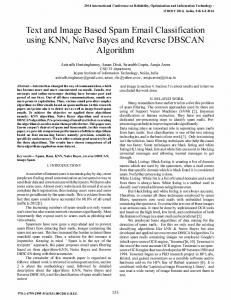
12. RESULTS AND INFERENCE The coding was done in C ; after the code was run, various performance measures such as the precision, recall, specificity & the accuracy, etc. were observed. The results are shown in the Figs. 8 to 11 respectively.

12.1 Precision

More the threshold, 4

5

BIRCH

Threshold

K-NNC

‘K’

Better the cluster quality & more number of centroids Lager the data & Higher the value of ‘K’, better classification results.

TABLE IV. EVALUATION MEASURES

True Positive True Negative False Positive False Negative

Test document Spam Non-Spam Spam Non-Spam

Classified to Spam Non-Spam Non-Spam Spam

BIRCH Phase 1 : Scan all data and build an initial CF tree.

Fig. 8 : Plot of measure of precision vs. data size Inference : The percentages of positive predictions that are correct are high for nearest neighbour classifiers. The precision table in table V and the following graph in Fig. 8 shows that for large data sets, BIRCH with NNC and K-means with NNC has an optimal value. TABLE V.

QUANTITATIVE RESUTLS OF PRECISION

Data

K-means

K-means

BIRCH

BIRCH

size

NNC

K-NNC

NNC

K-NNC

120

81.2%

72.9%

75%

61.9%

200

91.1%

74.4%

88.2%

91.6%

400

97.5%

56.6%

93.7%

69.8%

Phase 2 : Condense into desirable length by building a smaller CF tree. Phase 3 : Global clustering Phase 4 : Cluster refining (optional) - requires more passes over the data to refine the results 23

International Journal of Computer Applications (0975 – 8887) Volume 5– No.4, August 2010 K-NNC combination, which can also be observed from the Fig. 10.

12.2 Recall

12.4 Accuracy

Fig. 11 : Plot of measure of accuracy vs. data size

Fig. 9 : Plot of measure of recall vs. data size Inference : The percentage of positive labelled instances that predicted positive are high for the combination of K-means algorithm with K-NNC as the classifier and the percentage increases as the data set size increases. BIRCH does not work well for smaller data sets. The recall values can be visualized from the following table in table VI which indicates that for large data sets, BIRCH with K-NNC has a high value, which can also be observed from the Fig. 9. TABLE VI. QUANTITATIVE RESUTLS OF RECALL

Data size 120 200 400

K-means NNC 78.7% 97.6% 63.4%

K-means K-NNC 84.3% 97.6% 96.2%

BIRCH NNC 63.1% 71.4% 58.1%

BIRCH K-NNC 49.6% 52.3% 63.7%

12.3 Specificity

TABLE VIII.

Data size 120 200 400

QUANTITATIVE RESUTLS OF ACCURACY

K-means NNC 79.68% 94.4% 77.4%

K-means K-NNC 76.56% 82.14% 70.19%

BIRCH NNC 65.62% 80.9% 71.6%

BIRCH K-NNC 57.81% 73.8% 75.48%

Inference : Accuracy for BIRCH with K-NNC has a optimal value as the data set increases, also K-means works well for smaller data set. It can be visualized from the graph in Fig. 11 that conditions being checked hold good for large data and BIRCH with K-NNC is the best combination if the data set increases. It can be seen that BIRCH with K-NNC is more accurate for large data, which can be observed from the quantitative results shown in the table VIII. TABLE IX. COMPARISONS OF BIRCH & K-MEANS WITH DATASETS

BIRCH

K-means

Time

Faster

Slower

Sensitivity to input pattern of dataset

Yes

No

More

Less

Accurate

Accurate

Less

More

Cluster Quality (center location, number of data point in a cluster, radii of clusters) Demand for memory Fig. 10 : Plot of measure of specificity vs. data size TABLE VII. QUANTITATIVE RESUTLS OF SPECIFICITY

Data

K-means

K-means

BIRCH

size

NNC

K-NNC

NNC

K-NNC

120

80.6%

68.7%

69.2%

75%

200

90.4%

66.6%

90.4%

95.2%

400

97.6%

53.9%

93.6%

82.8%

BIRCH

Inference : The percentages of negative labelled instances that are predicted as negative are high for the combination using NNC as the classifier. The specificity values for large data sets as seen from the following table in table VII are optimal for BIRCH with

Finally, comparisons are made between Birch & K-means and the advantages / dis-advantages are shown in the table IX. It is concluded that BIRCH is the best when data-sets are taken into consideration.

13. Conclusions In this paper, an email clustering method is proposed and implemented to efficient detect the spam mails. The proposed technique includes the distance between all of the attributes of an email. The proposed technique is implemented using open source technology in C language; ling spam corpus dataset was selected for the experiment. Different performance measures such as the precision, recall, specificity & the accuracy, etc. were observed. K-means clustering algorithm works well for smaller data sets. 24

International Journal of Computer Applications (0975 – 8887) Volume 5– No.4, August 2010 BIRCH with K-NNC is the best combination as it works better with large data sets. In BIRCH clustering, decisions made without scanning the whole data & BIRCH utilizes local information (each clustering decision is made without scanning all data points). BIRCH is a better clustering algorithm requiring a single scan of the entire data set thus saving time. The work presented in this paper can be further extended & can be tested with different algorithms and varying size of large data sets.

REFERENCES [1] Sudipto Guha, Adam Meyerson, Nina Mishra, Rajeev Motwani and Liadan O’Callaghan, “Clustering Data Streams,” IEEE Trans.s on Knowledge & Data Engg., 2003. [2] Enrico Blanzieri and Anton Bryl, “A Survey of LearningBased Techniques of Email Spam Filtering,” Conference on Email and Anti-Spam., 2008. [3] Jain A.K., M.N. Murthy and P.J. Flynn, “Data Clustering : A Review,”ACM Computing Surveys., 1999. [4] Tian Zhang, Raghu Ramakrishnan, Miron Livny, “BIRCH: An Efficient Data Clustering Method For Very Large Databases,” Technical Report, Computer Sciences Dept., Univ. of Wisconsin-Madison, 1996. [5] Porter. M, “An algorithm for suffix stripping”, Proc. Automated library Information systems, pp. 130-137, 1980. [6] Manning C.D., P. Raghavan, H. Schütze, “Introduction to Information Retrieval”, Cambridge University Press, 2008. [7] Richard O. Duda, Peter E. Hart, David G. Stork, “Pattern Classification”, Wiley-Interscience Pubs., 2nd Edn., Oct. 26 2000. [8] http://www.informationretrieval.org/ [9] http://www.aueb.gr/users/ion/publications.html [10] http://www.cl.cam.ac.uk/users/bwm23/ [11] http://www.wikipedia.org [12] Jiawei Han and Micheline Kamber, “Data Mining Concepts and Techniques”, Second Edn. [13] Ajay Gupta and R. Sekar, “An Approach for Detecting SelfPropagating Email Using Anomaly Detection”, Springer Berlin / Heidelberg, Vol. 2820/2003. [14] Anagha Kulkarni and Ted Pedersen, “Name Discrimination and Email Clustering using Unsupervised Clustering and Labeling of Similar Contexts”, 2nd Indian International Conference on Artificial Intelligence (IICAI-05), pp. 703722, 2005. [15] Bryan Klimt and Yiming Yang, “The Enron Corpus: A New Dataset for Email Classification Research”, European Conference on Machine Learning, Pisa, Italy, 2004.

[16] Sahami M., S. Dumais, D. Heckerman, E. Horvitz, “A Bayesian approach to filtering junk e-mail”. AAAI’98 Workshop on Learning for Text Categorization, http://robotics.stanford.edu/users/sahami/papersdir/spam.pdf, 1998. [17] Sculley D., Gordon V. Cormack, “Filtering Email Spam in the Presence of Noisy User Feedback”, CEAS 2008: Proc. of the Fifth Conference on Email and Anti-Spam. Aug., 2008. [18] Dave DeBarr, Harry Wechsler, “Spam Detection using Clustering, Random Forests, and Active Learning”, CEAS 2009 – Sixth Conference on Email and Anti-Spam, Mountain View, California, USA, July 16-17, 2009. [19] Manning, C.D., Raghavan, P., and Schutze, H., “Scoring, Term Weighting, and the Vector Space Model”, Introduction to Information Retrieval, Cambridge University Press, Cambridge, England, pp. 109-133, 2008. [20] Naresh Kumar Nagwani and Ashok Bhansali, “An Object Oriented Email Clustering Model Using Weighted Similarities between Emails Attributes”, International Journal of Research and Reviews in Computer Science (IJRRCS), Vol. 1, No. 2, pp. 1-6. Jun. 2010. Mr. M. Basavaraju completed his Masters in Engineering in Electronics and Communication Engg. from the University Visvesvaraya College of Engg. (Bangalore), Bangalore University in 1990, & B.E. from Siddaganga Institute of Technology (Tumkur), Bangalore University in the year 1982. He has got a vast teaching experience of 23 years & an industrial experience of 7 years. Currently, he is working as Professor and Head of Computer science & Engg. Dept., Atria Institute of Technology, Bangalore, Karnataka, India. He is also a research scholar in Coimbatore Inst. of. Tech., Coimbatore, doing his research work & progressing towards his Ph.D. in the computer science field from Anna University Coimbatore, India, He has conducted a number of seminars, workshops, conferences, summer courses in various fields of computer science & engineering. His research interests are Data Mining, Computer Networks, Parallel computing. Dr. R. Prabhakar obtained his B. Tech. degree from IIT Madras in 1969, M.S. from Oklahoma State University, USA and Ph.D. from Purdue University, USA. Currently he is professor of Computer of Science and Engineering and Secretary of Coimbatore Institute of Technology, Coimbatore, India. His areas of specialization include Control Systems, CNC Control, Robotics, Computer Graphics, Data Structures, Compilers, Optimization. He has published a number of papers in various national & international journals, conferences of high repute. He has done a number of projects in the national & international level. At the same time, he has guided a number of students in UG, PG & in the doctoral level.

25