A novel multiple-controller incorporating a neural network based

© Neurocomputing (Elsevier Science) Volume 69, Issue 16, Pages 1868-1881 (October 2006)

1

A novel multiple-controller incorporating a neural network based generalized learning model Ali S. Zayed, Amir Hussain, Rudwan Abdullah Department of Computing Science and Mathematics, University of Stirling, FK9 4LA, Scotland, UK Tel: +44 1786-467437, Fax: +44 1786-464551 Corresponding author’s E-mail: [email protected]

Abstract A new adaptive multiple-controller is proposed incorporating a neural network based Generalized Learning Model (GLM). The GLM assumes that the unknown complex plant is represented by an equivalent stochastic model consisting of a linear time-varying sub-model plus a Radial Basis Function (RBF) neural-network based learning sub-model . The proposed non-linear multiple-controller methodology provides the designer (through simple switching) with a choice of using either a conventional Proportional-Integral-Derivative (PID) controller, a PID based pole-placement controller, or a PID based zero-pole placement controller. Sample simulation results using a realistic non-linear Single-Input Single-Output plant model are used to demonstrate the effectiveness of the proposed non-linear controller, with respect to tracking desired set-point changes, and it also illustrates the efficiency of employing the RBF neural network in representing the non-linear dynamics compared with conventionally used Multi-Layered Perceptron (MLP) neural networks.

Keywords: Multiple controllers, learning models, neural networks, PID control, zero-pole placement control.

1 Introduction In many industrial sectors, such as the steel, food, chemical and textile industries, the numerous deployed machines and processes can be improved through the use of optimal control and optimisation techniques. A difficult problem in the control of these industrial processes is due to the inherent complexity (that is, significant non-linearity, non-stationarity and uncertainty) of their models, which cannot be solved using traditional predictive or generalised minimum variance [1-2] based self-tuning control techniques. The application of linear control theory to these problems relies on the key assumption of a small range of operation in order for the (local) linear model assumption to be valid. When the required operating range is large, a linear controller may not be adequate. For this reason, it seems appropriate to extend generalised minimum variance control to complex


2

plants with non-linear models and with plant/model mismatch. A possible way to achieve this is by incorporating the inherent non-linearity of the process into the control design process using a learning model [14,19] “Learning models” result from a synthesis of learning systems. A learning system can be considered to be an adaptive system with memory, and “learning” then means that the system adapts to its current environment and stores this information to be recalled later. Thus, one may expect that a learning system improves its performance with time. Learning systems are particularly useful whenever complete knowledge about the environment is either unknown, expensive to obtain or impossible to quantify. When learning systems are synthesized with modelling techniques, so-called learning models emerge. Furthermore, when learning models are used with advanced control methods, they result in learning control systems [3, 14]. Over the last decade or so, there has been much progress in the modelling and control of non-linear processes, using black-box type learning models, such as neural networks [3, 4, 16, 19]. This is due to their proven ability to learn arbitrary non-linear mappings [4, 5]. Other advantages inherent in neural networks include their robustness, parallel architecture and fault tolerant capabilities. Neural networks have been shown to be very effective for controlling complex non-linear systems, when there is no complete model information, or when the controlled plant is considered to be a “black box” [3, 4, 5]. More recently, Zhu and Warwick [19] have proposed a more generalised method for developing non-linear adaptive control based on an input-output non-linear modeling framework. In such a design, which we term the Generalized Learning Model (GLM), the process model can be split into two parts, namely linear and non-linear dynamical sub-models, so that this special structure allows the linear part of the controller to exploit classical linear theory. On the other hand, the so called three-term proportional-integral-derivative (PID) controllers are still considered as the dominant controllers in the process control industries. The main reasons for this domination are summarised as follows [11, 12, 15]: 1.

PID controllers have simple control structures.

2.

It is relatively easy to understand the physical meanings of the control parameters.

3.

They are easy to implement using digital or analog hardware and are remarkably effective in regulating a wide range of applications once properly tuned.

However, these controllers may need to be re-tuned, if the systems to be controlled are subjected to some kind of disturbances in order to achieve satisfactory performance. For this reason, current trends in the field of


3

self-tuning control are towards incorporating the ability of automatic on-line tuning and utilising the simplicity of the PID controller structures, e.g. [10, 11, 12]. During the past three decades, a great deal of attention has been paid to the problem of designing polezero placement controllers and self-tuning regulators. Various self-tuning controllers based on classical poleplacement ideas were developed and employed in real applications, see e.g. [8, 9, 17, 19]. The popularity of pole-placement techniques may be attributed to the following [14, 16]: 1) In the regulator case, they provide mechanisms to over-come the restriction to minimum-phase plants imposed by the original minimum variance self-tuner of Astrom and Wittenmark [1]. 2) In the servo case, they provide the ability to directly introduce bandwidth and damping ratio as tuning parameters and unlike many of the self-tuning based PID control designs (see for example [11, 12]), in which the tuning parameters must be selected using a trial and error procedure. 3) Pole-placement methods are also known to be more robust compared to the early optimal self-tuning controllers as they aim to simply modify the system dynamics as opposed to cancelling them. 4) The arbitrary zeros may be used to achieve better set point tracking as shown in [14, 16] and may also help reduce the magnitude of the control action [9, 16].

In this paper, a new non-linear multiple-controller algorithm is developed which exploits the benefits of both the PID and pole-zero placement controllers within a GLM framework. The proposed design builds on the previous works of Zayed et al. [14, 17], by investigating the applicability of the GLM based multiple-controller methodology for complex plants. The parameters of the linear sub-model are identified by a standard recursive identification algorithm, and a conventional multi-layered neural network is utilised as the non-linear learning sub-model. The main contribution of this paper is in the development of a new GLM based multiple controller, which provides the designer (through a simple switch) with the choice of using either a PID self-tuning controller, a PID pole-placement controller, or a newly proposed PID pole-zero placement controller. All controllers operate using the same adaptive procedure and a selection between the various controller options is made on the basis of the required performance measure. The switching (transition) decisions between the various controllers can be automated using, for example, Stochastic Learning Automata of [7]. However, in the present case, a manual switching mechanism has been adopted to demonstrate the feasibility of the developed approach. Another contribution is to use RBF neural networks for approximating the non-linear sub-model instead of the MLP neural networks in order to achieve more efficient closed loop system performance.


4

The paper is organised as follows: the derivation of the control law for the proposed multiple controller is discussed in section 2. In section 3, a detailed simulation case study is carried out in order to demonstrate the effectiveness of the proposed multiple controller framework with respect to tracking set point changes. In order to compare the robustness of the new multiple controller framework, which employs the RBF neural network, with that of Zhu and Warwick [19], the variance of the closed loop system and/or control input is used to asses the performance. Finally, a discussion on the selection of the multiple controller modes and switching issues, together with some concluding remarks, are presented in section 4.

2. Derivation of the control law Consider the following representation for nonlinear plant model [14, 17, 19]:

A( z −1 ) y (t + k ) = B( z −1 )u (t ) + f 0,t (Y,U ) + ξ (t + k )

(1)

where y (t ) is the measured output, u (t ) is the control input and ξ (t ) is uncorrelated sequence of random

variables with zero mean at the sampling instant t = 1,2,... , and k is the time delay of the process in the integer-sample interval. The term f 0 ,t (Y,U) in equation (1) above, is potentially a non-linear function (which accounts for any unknown time-delays, uncertainty and non-linearity in the complex plant model). The overall plant model represented by equation (1) above, is also known as the Generalized Learning Model (GLM) [14], and can be seem as the combination of a linear sub-model and a non-linear (learning) sub-model as shown in Figure (1).Also, in equation (1), we define y(t) ∈ Y , and u(t) ∈ U ; {Y ∈ R n a ; U ∈ R nb } and A(z −1 ) and B(z −1 ) are polynomials with orders n a and nb , respectively, which can be expressed in terms of the backwards shift operator, z −1 as: A(z −1 ) = 1 + a1 z −1 + ....,.... + an a z − n a

(2a)

B(z −1 ) = b0 + b1 z −1 + ....,.... + bnb z − nb , b0 ≠ 0

(2b)

It can be seen from equations (2a) and (2b) that the equivalent linear sub-model is devised by assuming that no coupling relationships exist. As stated earlier, the non-linear relationships are meanwhile accommodated in the nonlinear part f 0 ,t(.,.) . In order to simplify the analysis, the time delay is taken as k = 1 [17]. For this case the non-linear system represented by equation (1) can be written as [14, 19]:


A(z −1 )y(t) = z −1B(z −1 )u(t) + z −1 f 0 ,t(Y,U) + ξ(t)

5

(3)

The generalised minimum variance controller of interest minimises the following cost function [14, 19]: J N = E{[φ{[ + 1 )]}

(4)

where φ(t + 1 ) = [P(z −1 )y(t + 1 ) + Q(z −1 )u(t) − R(z −1 )w(t) − H N (z −1 )f 0 ,t(.,.)]

(5)

where w(t) is a bounded set point and P(z −1 ) = [Pd (z −1 )] −1 Pn(z −1 ), Q(z −1 ) , R(z −1 ) and H N (z −1 ) are userdefined transfer functions in the backward shift operator z

−1

and E{.} is the expectation operator.

Next, we can introduce the following identity [17]:

Pn(z −1 ) = A(z −1 )E(z −1 )Pd (z −1 ) + z −1 F(z −1 )

(6)

where E(z −1 ) , F(z −1 ) , Pn(z −1 ) and Pd (z −1 ) are polynomial in z −1 . where Pn(z −1 ) and Pd (z −1 ) are the numerator and denominators of the polynomial matrix P(z −1 ) . The orders of the polynomial matrices E(z −1 ) , F(z −1 ) and Pn(z −1 ) in the equations (6) are specified as follows:

ne = k − 1 n f = (n Pd + n a − 1) n pn = max(n a + n pd + n e , k + n f )

    

(7)

where, n f , n pn and n pd represents the degrees of Pd (z −1 ) , Pn(z −1 ) and Pd (z −1 ) respectively. Multiplying (3) by Pd (z −1 )E(z −1 ) and substitute for ( E(z −1 )A(z −1 ) ) from equation (6) gives: [Pd ] −1 Pn y(t + 1 ) = F(z −1 )y(t) + B(z −1 )E(z −1 )u(t) + Ef 0 ,t (.,.) + Eξξ( + 1 )

(8)

Adding Q(z −1 )u(t) − R(z −1 )w(t) − H N (z −1 )f 0 ,t (.,.) to both sides of equation (8) and using equation (6), yields: φ(t + 1 ) = [Pd (z −1 )] −1 F(z −1 )y(t) + (Q(z −1 ) + B(z −1 )E(z −1 ))u(t) − R(z −1 )w(t) +

(E(z −1 ) − H N (z −1 ))f 0 ,t (.,.) + E(z −1 )ξξ( + 1 ) In the rest of this section, the argument

(9)

z −1 will be omitted from various polynomials and transfer functions in

order to simplify the notation and only be used where required for clarification purposes. ~ Now we can define the optimal predictor φ*(t + 1|t) and the prediction error φ (t + 1 | t ) as follows:

φ*y(t + 1|t) = [Pd ] −1 Fy(t) + (Q + EB)u(t) + [E − H N ]f0 ,t (.,.)

(10)


~ (t + 1|t) = Eξξ( + 1 ) φ

6

(11)

If we set φ*(t + 1|t) = 0 in equation (10) and after some arrangement, the generalised minimum variance control law for non-linear systems is obtained as: Pd (EB + Q)u(t) = [Pd Rw(t) − Fy(t) + Pd (H N − E)f 0 ,t(.,.)]

(12)

Now, if we set: R = [Pd ] −1 H 0 H N = ([Pd ] −1 ∆H ′N + E)

  

(13)

next, if we set the transfer function Q(z −1 ) such that the following relation is satisfied [14, 17]: Pd (EB + CQ) = v −1 ∆q′

(14)

then, equation (12) becomes: ∆q′u(t) = [vH 0 w(t) − v(F)y(t) + ∆vH ′N f 0 ,t(.,.)]

(15)

where v is a user defined gain [10, 11] and q′ is a polynomial in z −1 having the following form:

q′(z −1 ) = 1 + q1′ z −1 + ............. + q′n ′ z

− n q′

q

(16)

where n q′ is the degree of the polynomial q′ . We can see clearly from equations (14) and (15) that the controller denominator has now conveniently been split into two parts: 1) An integrator action part ( ∆ ) required for PID design. 2) An arbitrary compensator ( q′ ) that may be used for pole-placement and pole-zero zero placement design. It can be seen from equation (14) that the polynomial matrix q′(z −1 ) and the gain matrix V are user-defined parameters since they depend on the user transfer function Q(z −1 ) . It is also clear from equation (13) that H 0 and H ′N are user-defined parameter because they depend on the transfer functions R( Z −1 ) and H N respectively. Now, if we set: ~ ~ H 0 = H [ H (1)]−1 F (1)

(17)


7

and combine equations (17) and (15), then we can readily obtain: ~ ~ ∆q′u(t) = vH[H( 1 )] −1 F( 1 )w(t) − v(F)y(t) + ∆vH N′ f 0 ,t (.,.)

(18)

~ where H in equation (18) is a user-defined polynomial which can be used to introduce arbitrary closed loop

zeros for explicit pole-zero placement controller and has the following form: ~ ~ −n ~ H(z −1 ) = 1 + h1 z −1 + ...... + hn~ z

(19)

h

The above equation (18) represents the final expression of the control law for the proposed non-linear MIMO multiple controller.

2.1 Multiple Controller Mode 1: Conventional non-linear PID controller

In this mode, the so-called multiple controller operates as a conventional self-tuning PID controller, which can be expressed in the most commonly used velocity form [11, 15] as: ∆u(t) = K I w(t) − [K P + K I + K D ]y(t) − [ − K P − 2 K D ]y(t − 1 ) − K D y(t − 2 )

(20)

If we assume that the degree of F(z −1 ) is equal to 2 F ( z −1 ) = f 0 + f1 z −1 + f 2 z −1

(21)

~ and switch both of pole-placement polynomial q′ given by equation (16) and zero-placement polynomial H

given by (19) off by setting: q′(z −1 ) = 1, (i.e. q1′ = q′2 = ..,.. = qn ′ = 0 ) q ~ ~ ~ ~ H = 1, (i.e. h1 = h2 = ...,... = hn ~ = 0 ) h

   (22a) 

next, if we set: H N′ = −(B( 1 )v)−1q′( 1 )

(22b)

then a self-tuning controller with PID structure is obtained, where ∆u(t) = [vF( 1 )w(t) − v(f 0 + f1 z −1 + f 2 z −1 )y(t) + ∆vH ′N f 0 ,t (.,.)]

(23)

K P = −v f1 + 2v f 2

(24a)

K I = v f 0 + v f1 + v f 2

(24b)

© Neurocomputing (Elsevier Science) Volume 69, Issue 16, Pages 1868-1881 (October 2006) KD = v f2

8

(24c)

It can be seen from the above equations (23), (24a), (24b) and (24c) that the PID control parameters K P , K I and K D depend on the polynomial matrix F(z −1 ) and the gain v [11, 12]. In this case the parameters of the polynomial matrix F(z −1 ) , f 0 , f1 and f 2 are computed directly from the equation (6) by selecting suitable user-defined polynomials Pd and Pn which are selected in trial and error basis [11, 12]. It can also clearly be seen from equation (7) that the order of F(z −1 ) which indicates the type of the controller (PI or PID) is governed by the polynomial A and Pd [11, 12]. As stated above the multiple controller mode 1 described by equations (20)-(24c) is tuned by a selection of the polynomials Pn and Pd , and the gain v . However, the main disadvantage of many PID self-tuning based minimum variance control designs (see for example [11, 12]) is that the tuning parameters must be selected using a trial and error procedure. Alternatively, these tuning parameters can be automatically and implicitly set on line by specifying the desired closed loop poles [6, 14, 19].

2.2 Multiple Controller Mode 2: Nonlinear PID based pole placement controller Substituting for u(t ) given by equation (18) into the process model described by equation (3), the closed loop system is obtained as: ~ ~ ~ (A q′ + z −1B F)y(t) = z −1 BvH[H( 1 )] −1 F( 1 )w(t) + ∆(z −1BvH N′ + q′)f 0 ,t + ∆q′ξ(t)

(25)

where

~ A = ∆A  ~ B = VB 

(26)

We can now introduce the identity: ~ ~ (q ′A + z −1 FB ) = T

(27)

where T is the desired closed loop poles and q′ is the controller polynomial. For equation (27) to have a unique solution, the order of the regulator polynomials and the number of the desired closed loop poles must be set as [8, 14, 16]:

© Neurocomputing (Elsevier Science) Volume 69, Issue 16, Pages 1868-1881 (October 2006)     

n f ′ = n a~ − 1 = n a n q′ = nb~ + k − 1 nt ≤ n a~ + nb~ + k − 1

9

(28)

~ ~ where na~ , nb~ , and n q′ are the orders of the polynomials A, B and q′ , respectively, and nt denotes the number of desired closed loop poles. Also, nb~ = nb and n a~ = n a + 1. Combining equations (25) and (27), gives: ~ Ty(t) = z −1 BvH[H( 1 )] −1 F( 1 )w(t) + ∆(z −1 BvH N′ + q′)f 0 ,t + ∆q′ξ(t)

(29)

If the explicit zero placement polynomial given by (19) is switched off by setting: ~ ~ ~ ~ H = 1, (i.e. h1 = h2 2 = ...,... = hn ~ = 0

(30)

h

And, if we set:

H ′N = −(B( 1 )v)−1q′( 1 )

(31)

then the closed loop function of equation (29) becomes:

Ty(t) = z −1BvF( 1 )w(t) + ∆(z −1Bvq′( 1 )[ − (B( 1 )v)−1 ] + q′)f 0 ,t ∆q′ξ(t)

(32)

In this case: T( z −1 ) = 1 + t1 z −1 + t2 z −2 + .......... + t nt z − nt

where n h~

and nt

(33)

in equations (30) and (33) represent orders of the polynomials

~ H(z −1 ) and

T(z −1 ) respectively. It can be seen from equation (32) that the closed loop poles are placed at their desired positions which is prespecified by the user through the use of the polynomial T(z −1 ) .

2.3 Multiple Controller Mode 3: Nonlinear PID based zero-pole placement controller

In this controller mode, an arbitrary desired zeros polynomial can be used to reduce excessive control action, which can result from set point changes when pole placement is used.

© Neurocomputing (Elsevier Science) Volume 69, Issue 16, Pages 1868-1881 (October 2006) 10 ~ If the zero-placement polynomial ( H ) given by equation (19) is switched on then the closed loop given by

equation (25) is again obtained and can be simplified as follows: then the closed loop function of equation (32) becomes: ~ ~ Ty(t) = z −1 Bv[H( 1 )] −1 HF( 1 )w(t) + ∆(z −1 Bvq′( 1 )[ − (B( 1 )v)−1 ] + q′)f 0 ,t + ∆q′ξ(t)

(34)

~ Note that in practice, the order of T(z −1 ) and H(z −1 ) are most of the time selected to equal 1 or 2 [9, 16]. It can be seen from equations (34) that the closed loop poles and zero are placed at their desired positions which ~ pre-specified by using the polynomials T(z −1 ) and H(z −1 ) . Clearly from equations (6)-(7) and (12)-(16) above, the user defined transfer functions P , Q , R and H N must change at every sampling instant in order to satisfy the conditions specified by equations (21), (22), (24a), (24b) and (24c) for achieving self-tuning PID control (multiple controller mode 1). On the other hand, the above under defined transfer functions must change in order to satisfy equations (27), (28) (30) (31) and (33) for achieving pole-placement control (multiple controller mode 2). Finally, for achieving pole-zero placement control (multiple controller mode 2) these user-defined transfer functions must change automatically in order to satisfy equations (27), (28), (31) and (19). However, note that it is not necessary to explicitly calculate these user defined design transfer functions [14, 16, 17]. This does of course, suggest that the cost index has time varying weightings in this problem. In the next section, the identification of complex non-linear plants using the GLM framework is discussed.

2.4 Generalized Learning Models (GLM) for identification of plants

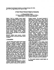
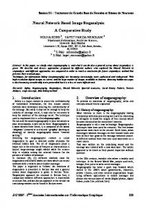
As can be seen in figure (1), a recursive least squares algorithm is initially used to estimate the parameters A and

B (equation (3)) of the linear sub-model. Then an artificial neural network is used to approximate the non-linear part f 0, t . The Back Propagation (BP) Multi Layer Perceptron MLP and Radial Basis Function (RBF) neural networks are experimented to achieve accurate nonlinearity representation. (which accounts for any uncertainty, time-varying and non-linear multi-variable interactions in the complex plant model) It can be seen from equation (3) that the ith measured output yi (t ) can be obtained as follows:

yi (t + 1) = ϕiT (t )θ i (t ) + f 0, i (y , u ) where

(35)

© Neurocomputing (Elsevier Science) Volume 69, Issue 16, Pages 1868-1881 (October 2006) 11

and i = 1,2,......, n where

(36)

y(t) = [y1(t), y2(t),......,yn(t)] T

is

the

measured

output

vector

with

dimension

(n × 1)

and

u(t) = [u1(t), u2(t),......,u n(t)] T is control input vector. where θi is the parameter vector and ϕ i ∈ ℜ m is the data vector as follows:

  [yi(t − 1 ),.......,yi(t − na ),ui(t − 1 ),.....ui(t − nb )] 

θi(t) = [ − a1,i ,............, − an a,i ,b0 ,i ,......,bnb,i ] T

ϕiT (t) =

(37)

Equation (3) and (35) can also be presented as:

yi(t) = yˆ i(t) + f 0 ,i(.,.)

(38)

ˆ It is clear from Figure (1) that yˆ i(t) = ϕ iT (t)θˆi(t) is the linear sub-model output and f 0 ,i(.,.) = yi(t) − yˆ i(t) is the difference between the actual output yi (t ) and the linear sub-model output ~ yˆ i (t ) . From Figure (1) we can also see that f 0, i (.,.) can be expressed as:

f 0,i (.,.) = f 0,i + εi (t )

(39)

Using the above equation (39) and as can be seen in Figure (1), a neural network is used for estimating the nonlinear function f 0,i , with the identification error

ε i (t ) being used to update the weights and thresholds of the

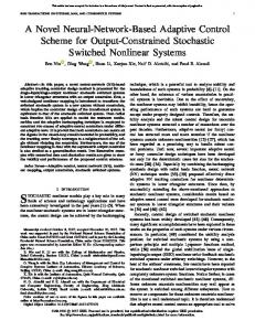
learning neural network model. The neural network model employed in the proposed control scheme is chosen to be a Radial Basis Function (RBF) neural network for its ability to represent the non-linear dynamics of the plan more accurately than the Back Propagation (BP) Multi Layer Perceptron MLP used by Zhu and Warwick [19], which shows inaccurate results when sudden changes in reference signal occur or disturbances arise. The schematic diagram of the ith neural network is shown in Figure (2). The non-linear function f 0(.,.) is adaptively estimated by using the following equations [14, 17]: 1

f 0,t (.,.) =

(40)

n

1 + exp[− β (

∑w g j

j

+ b)]

j =1

δ w = ηg j ,t f 0,t [1 − f 0,t ][ ~x (t ) − f 0,t ]

(41)

w j (t ) = w j (t − 1) + δ w

(42)

© Neurocomputing (Elsevier Science) Volume 69, Issue 16, Pages 1868-1881 (October 2006) 12 2  i  l xi − c j g 0,t (.,.) = exp − ∑ 2  i =1 2σ ij 

( )

    

(43)

Where w j is the hidden layer weights, β is the output layer threshold, δ w is the change in weights, η is the learning rate,

xi is the inputs, c ij is the mean, l = n a + nb , and g j is the output of the hidden layer. The

variance of the Gaussian units σ ij is dependent on the input dimension because the RBF inputs are scaled differently [10].

The overall adaptive multiple controller framework is illustrated in Figure (1).

PID Controller

switch

Manual /Stochastic Learning Automata u(t)

PID pole Placement controller

y (t ) Plant

controller Switch between Non-linear Controller Modes

PID pole-zero Placement controller

+ GLM Linear submodel

yˆ (t ) −

ε(t )

f 0(.,.) − f 0(.,.)

GLM Non-linear SubModel (employing a Neural Network predictor)

+ Set-point:w (t ) R

+ −

Figure (1): Proposed non-linear adaptive multiple controller framework incorporating a Neural Network based Generalized Learning Model (GLM)

b = 1

g1

w1 g

w

2

U

∑ w

Y

g

Input layer

2

f 0 ,t

n

n

Hidden layer

Output layer

Figure (2): Neural network learning model to approximate the non-linear function f 0,t (.,.)


2.5 Nonlinear multiple-controller algorithm summary The proposed multiple controller can now be summarised as: ~ Step 1. Select the desired closed-loop system poles and zeros polynomials T and H (for explicit pole-zero

control). Step 2. Select Pd , Pn and v for conventional PID control. Step 3. Read the current values of y(t ) and w (t ). Step 4. Estimate the process parameters Aˆ and Bˆ using a conventional exponentially weighted RLS algorithm [1,15]. Step 5. In order to switch to the conventional PID controller (multiple controller mode 1), then following steps must be followed: Step (5.1) Compute Fˆ from equation (6) using the polynomials Pd and Pn and the gain v selected in step 2. ~ Step (5.2) set qˆ ′ = 1 , H = 1 and H ′N = −(B( 1 )v)−1q′( 1 ) using equations (22a) and (22b). Step 6. In order to switch to the PID pole-placement controller (multiple controller mode 2) then compute Fˆ and ~ qˆ ′ using (26) and (27) and switch off the explicit zero placement polynomial by setting H = 1 using

(30). Step 7. In order to switch to the PID pole-zero placement controller (multiple control mode 3) then compute Fˆ ~ and qˆ ′ using (26) and (27), and switch on the pole-zero placement polynomial H using (19).

Step 8. Compute f 0(.,.) = y(t) − yˆ (t) , where yˆ (t) is the output of the linear sub-model. Step 9. Apply the neural network to obtain f 0 ,t (.,.) by using equations (40)-(43). Step 10. Compute the control input using (18). Steps 3 to 10 are to be repeated for every sampling instant.

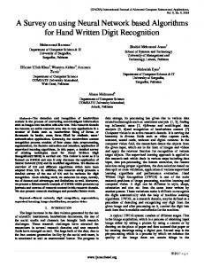
© Neurocomputing (Elsevier Science) Volume 69, Issue 16, Pages 1868-1881 (October 2006) 14 3. Simulation results The objective of this section is to study the performance and the robustness of the closed loop system using the multiple-controller framework proposed in Section 2. A simulation case study will be carried out to demonstrate the ability of the proposed algorithm to adaptively locate the closed-loop poles and zeros at their desired locations under set point changes. In chemical process industries, one of the most commonly occurring control problems is that of controlling the fluid levels in storage tanks or reaction vessels. In this example, the proposed controller is applied to a real world system model shown in Figure (3) and described in detail in [16]. The tank system illustrated in Figure (3) is 10cm long, 10cm deep and 30cm high. The main objective of the control problem is to adjust the inlet flows

f L1 so as to maintain the level in the tank hs1 as close to a desired set point with desired closed

performance. The fluid flow rate into the tank

( f L1 ) is supplied by a pump. To measure this flow rate, a flow

meter is inserted between the pump and the tank. The flow of water from the tank to reservoir

( f L0 ) is

controlled by an adjustable tap. The maximum diameter of this tap is 0.70 cm. The depth of fluid is measured using a parallel track depth sensor which is located in the tank. The non-linear model can be presented as follows [16]:

A

dhs1 dt

where

= f L1 − a1′ σ1 2 g (hs1 − hs 2 )

(44)

a1′ is the cross section area of orifice, σ1 is the discharge coefficient (0.6 for a sharp edged orifice) [15],

and g = 9.81 N / m 2 . The diameter of orifice is adjusted to 0.95cm and drain valve is fully open. The set point w(t ) changes every 100 samples between 15m and 20m during a period of 600 samples. A first order linear model [1 + Aˆ1 z −1 ] y1 (t ) = z −1 Bˆ 0u (t ) is used to identify the parameters of the process using

RLS estimator. An RBF neural network shown in the Figure (2) is used to approximate the non-linear function ( f 0, t (.,.)). Pump1

f L1

a′1 hs 1 h′s f L0

Figure Water-tank Figure(5.6). (3): Water tank system


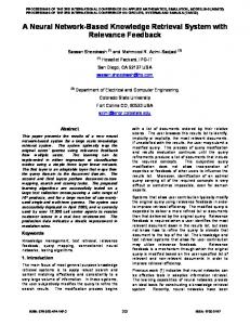
In order to implement the multiple controller algorithm the steps summarised in section (2.5) are followed. The user defined gain and the user-defined polynomials are respectively selected as: v = 1 , Pd (z −1 ) = I + Pd1 z −1 and Pn(z −1 ) = 1 + pn1 z −1 . where Pd1 = −0.8 and Pn1 = −0.5 . The desired closed ~ The closed loop poles and zeros are respectively selected as: T = 1 + −0.6 z −1 and H = 1 + 0.8 z −1 . It is clear from equations (6), (7), (28), (24a), (24b) and (24c) that a PI control structure is achieved. In order to demonstrate the closed loop performance of the multiple controller we arrange manually the PI based multiple-controller to work in all three control modes: namely as a PI self-tuning controller, PI pole-placement controller and as a PI pole-zero placement controller as described below: a) From 0th up to 200th sampling time, the conventional PI self-tuning controller is selected to operate on-line. b) PI pole placement controller is switched on from 201st to 400th sampling instant. c) The PI pole-zero placement controller is switched on from 401st to 600th sampling time. The experimental results shown in the following figures are to demonstrate three main objectives of this paper. Firstly, the effectiveness of including the non-linear sub-model, using the RBF neural network, in the plant model and accommodating it in the multiple controllers law. Figure (4a) and Figure (4b) respectively illustrate the system output signal hs (in meters) and input signal f L1 in (m 3 / sec) where the non-linearity dynamics 1 were included in the design of the plant model and accommodated within the multiple controllers law. Figure (5a) and figure (5b) respectively show the system output signals and input signals where only the linear behaviour of the plant was considered. From these results it can be seen that the resulting output signals during each of the three controllers session has better reference signal tracking and lower signal variance when the nonlinearity were included. Secondly, using the RBF neural network instead of the MLP neural networks shown more improved results in the output and input signals at the changes of the reference signal w (t ) is changing and when the disturbances were added. Figure(6a) presents the output signal while the RBF Neural network is used, figure (6b) shows lower variance input signal which led to the lower variance output signal than results presented in figures (7a) and (7b) when the MLP neural network is used to represent the non-linear sub-model of the plan. Thirdly, it can be seen from these figures (4 to 7) that, the transient responses are significantly shaped by the choice of the polynomial T when either a PI pole-placement controller or a PI zero-pole placement is used. It can also clearly be seen that excessive control action, which resulted from set-point changes, is tuned most effectively when the user selected PI zero-pole placement controller is operating on-line.


Also note that during the first 200 samples, where the conventional self tuning PI controller is operating, oscillations can be seen in the control input and closed loop output, hence exhibiting the worst performance as expected, due to its inherent limitations. The other disadvantage of the self-tuning PID controller is that the tuning parameters must be selected using a trial and error procedure.

PID Controller

PID Pole Placement Controller

Variance: 10.8341

Variance: 5.8017

PID Pole Zero Placement Controller Variance: 5.7921

Overall Variance: 7.4761

Figure (4a): The output signal when the non-linear sub-model is included

PID Controller


Variance: 6.9397

Variance: 0.8695



Figure (4b): The input signal when the non-linear sub-model is included


PID Controller


Variance: 10.6794

Variance: 6.1876



Figure (5a): The output signal when only the linear sub-model is used to model the plant

PID Controller


Variance: 12.9847

Variance: 1.0199



Figure (5a): The input signal when only the linear sub-model is used to model the plant


PID Controller


Variance: 11.1345

Variance: 5.9100



Figure (6a): The output signal when the RBF is used to represent the nonlinear sub-model of the plant

PID Controller


Variance: 6.9664

Variance: 1.2518



Figure (6b): The input signal when the RBF is used to represent the nonlinear sub-model of the plant


PID Controller


Variance: 11.3789

Variance: 7.1622



Figure (7a): The output signal when the MLP is used to represent the non-linear sub-model of the plant

PID Controller


Variance: 7.0344

Variance: 2.2697



Figure (7b): The input signal when the MLP is used to represent the nonlinear sub-model of the plant

5. Discussion and conclusions 5.1 Discussion on selection of controller type and switching issues

Due to the robustness, simplicity of structure, ease of implementation, and remarkable effectiveness in regulating a wide range of processes (assuming they are properly tuned), the conventional self-tuning PID controller proposed in section (2.1) is the first choice for a designer in order to obtain satisfactory closed-loop system performance.


If however, a better closed loop system performance (based on say, a desired damping ratio, rise time, settling time overshoot or bandwidth) is required, or if the system to be controlled is difficult to tune using a conventional self-tuning PID controller, then the PID pole-placement proposed in section (2.2) can be used. However this will be at the expense of a greater computational effort required for implementing the PID poleplacement controller. Finally, in the situation where an excessive control action results from use of the PID poleplacement controller, the multiple controller should be switched to operate in the PID pole-zero placement mode proposed in section (2.3), in order to obtain a more efficient control action, but at the expense of a greater computational requirement. 5.2 Conclusions

In this paper, a new non-linear multiple-controller algorithm is developed which combines the benefits of both the PID and pole-zero placement controllers within a novel GLM framework. The proposed methodology provides the designer with the choice of using a conventional PID self-tuning controller, a PID pole placement controller or the proposed PID pole-zero placement controller. All developed controllers operate using the same adaptive procedure and are selected on the basis of the required performance measure. The switching (transition) decision between these different fixed structure controllers was achieved manually in the present case. In the future it will be implemented using the Stochastic Learning Automata criterion proposed by [7]. Sample simulation results using a realistic plant model are used to demonstrate its effectiveness of using the RBF neural network to represent more accurately the behaviour and dynamics of the system. Furthermore, the results indicate that the PID pole-zero placement controller option provides the best set point tracking performance with the desired speed of response, but at the expense of a relatively greater computational requirement (compared to the other controller options). This particular controller option penalises the excessive control action most effectively, and it can also deal with non-minimum phase systems. The controller’s transient ~ response is shaped by the choice of the pole polynomial T(z −1 ) , while the zero polynomial H(z −1 ) can be used to reduce the magnitude of control action, or to achieve better set point tracking [9, 14, 16], compared to the computationally less expensive PID pole-placement and conventional self-tuning PID controllers.

Acknowledgements

This work was part-funded by the UK Engineering & Physical Sciences Research Council (EPSRC) Cluster Project Towards Multiple Model based Learning Control Paradigms for Complex Systems (Research Grant Ref. GR/S63779/01). The authors are indebted to Professor Mike Grimble of the Industrial Control Centre, University of Strathclyde, Glasgow (UK) for highly stimulating discussions and his insightful comments and suggestions.


References

[1] K. J. Astrom and B. Wittenmark, On self-tuning regulators, Automatica, 9 (1973) 185-199. [2] D. W. Clarke and P.J. Gawthrop, 1979, Self tuning control, Proc. Inst. Electrical Engineering, Part D, 126 (1979) 633-640. [3] R. Gomez, E. K. Najim and E. Ikonen, Stochastic learning control for non-linear systems, Intern. Joint Conf. on Neural Networks, Honolulu, Hawaii, U.S.A, 12-17, May 2002. [4] A. Hussain, J. Soraghon and T. Durrani A new adaptive Functional-link Neural Network Based DFE for Overcoming Co-Channel Interference, IEEE Transactions on Communications, 45 (10) (1997) 1358-1362 [5] A. Hussain, A. S. Zayed and L. S. Smith, A New Neural Network and pole placement Based Adaptive composite self-tuning, Proceedings of the fifth IEEE International Multi-topic Conference (INMIC,2001), Lahore, pages 267-271, 28-30 December, 2001. [6]

Z. Ma, A. Jutan and V. Baji, Non-linear Self-tuning Controller For Hammerstein Plants with application to a pressure tank, IJCSS, 1(2) (2000) 221-230

[7] K. Narendra, Thathachar M.A.L., Learning Automata, An Introduction, (Prentice-Hall, 1989). [8] D. Prager and P. wellstead, Multivariable pole-placement Self-tuning regulators, Proc. Inst. Electr. Engineering, Part D, 128 (1980) 9-18. [9] R. Sirisena and F. C. Teng, Multivariable pole-zero placement self-tuning controller, Int. J. Systems Sci., 17(2) (1986) 345-352. [10] M. Tokuda and T. Yamamoto, A neural-Net Based Controller supplementing a Multiloop PID Control System, IEICE Trans. Fundamentals, Vol. E85-A (1) (2002) 256-261. [11] R. Yusof, S. Omatu and M. Khalid, Self-tuning PID control: a multivariable derivation and application, Automatica, 30 (1994) 1975-1981. [12] R. Yusof and S. Omatu, A multivariable self-tuning PID controller, Int. J. Control. 57 (1993) 1387-1403. [13] W. Yu and A. Pozilyak, Indirect adaptive control via parallel dynamic neural networks, IEE. Proc. Control theory Appl., 146 (4) (1999) 25-30. [14] A. Zayed, Hussain A and M. Grimble, Novel non-linear Multiple-Controller framework for SISO Complex Systems incorporating a Learning sub-model, invited paper, in press, Int. J. of Control & Intelligent Systems, 33, (2005). [15] A. Zayed, MinimumVariance Based Adaptive PID Control Design, M.Phil Thesis, Industrial Control Centre, University of Strathclyde, Glasgow, U.K., 1997.


[16] A. Zayed, A. Hussain and L. Smith, A New Multivariable Generalised Minimum-variance Stochastic Selftuning with Pole-zero Placement, Int. J. of Control & Intelligent Systems, 32 (1) (2004) 35-44. [17] A. Zayed and A. Hussain, A New Non-linear Multi-variable Multiple-Controller incorporating a Neural Network Learning Sub-Model, in Proceedings of International Symposium on Brain Inspired Cognitive Systems (BICS2004), Stirling, 29 Aug - 1 Sep 2004. [18] A. Zayed and A. Hussain, Stability Analysis of a New pole-zero placement controller Neural Networks, Proc. 7th IEEE international multi-topic Conference (INMIC’2001), Lahore, 28-31 Dec 2003, 267-271. [19] Q. Zhu, Z. Ma and K. Warwick, Neural network enhanced generalised minimum variance self-tuning controller for nonlinear discrete-time systems, IEE Proc. Contol Theory Appl., 146(4) (1999) 319-326. [20]

A. Allidina and H. Yin, Explicit pole-assignment self-tuning algorithms, Int. J. Control, 42, 1985, 11131130.

[21] K. Passino, Biomimcry for Optimization, Control, and Automation, (Springer 2005).

A novel multiple-controller incorporating a neural network based

A novel multiple-controller incorporating a neural network based

Suggest Documents

A novel multiple-controller incorporating a neural network ... - CiteSeerX

A Novel Neural Network Based on Immunity

A novel wavelet neural network based pathological stage detection ...

A Novel Neural Network-Based Technique for Smart Gas ... - MDPI

A Novel Neural-Network-Based Adaptive Control ... - IEEE Xplore

A Novel Neural Network Based Method Developed for Digit ...

NEURAL NETWORK WORLD: A NEURAL NETWORK BASED ... - NNW

A Novel Active Semisupervised Convolutional Neural Network

A Neural Population Model Incorporating

A Neural Population Model Incorporating

tor vergata university novel neural network-based

A WAVELET BASED NEURAL NETWORK FOR ... - CiteSeerX

A Survey on using Neural Network based

A Neural Network-Based Knowledge Retrieval ...

A WAVELET BASED NEURAL NETWORK FOR ... - CiteSeerX

A Neural Network Based Model for Detecting

A Polynomial Neural Network Classifier based on

A Neural Network-Based Cryptographic System

A Neural Network-Based Four Phases Interleaved

A neural network-based intelligent metasearch engine

Neural Network Based Image Steganalysis: A ... - CiteSeerX

A Deep Convolutional Neural Network Based

Incorporating Side Information into Recurrent Neural Network ...

MINNI: Micromouse Incorporating Neural Network Intelligence Jondarr ...