ISSN 2278-3083 Volumeand 5, No.4, July -Information August 2016 M. Gooroochurn et al,, International Journal of Science Advanced Technology, 5 (4), July – August 2016, 14-27
International Journal of Science and Applied Information Technology Available Online at http://www.warse.org/IJSAIT/static/pdf/file/ijsait01542016.pdf
A Polynomial Neural Network Classifier based on Gabor Features for the Extraction of Ear Tragus and Eye Corners M. Gooroochurna, D. Kerrb, K. Bouazza-Maroufb
[email protected],
[email protected],
[email protected] a
b
Mechanical and Production Engineering Department University of Mauritius, Reduit, Mauritius
Wolfson School of Mechanical and Manufacturing Engineering Loughborough University, Loughborough, UK
methods [23-27] and neural network solutions [6-8, 19, 20, 28] have taken first stage in favour of methods employing decision rules based on geometry/symmetry of features extracted by grey-level processing, e.g. corners, edges, ridges and contours [29]. The reason for this shift in the design of face processing solutions is the ability to use large training sets for machine learning, which have given very good performance results, whereas methods relying solely on decision rules perform well only when operating conditions such as illumination, scale and rotation are closely controlled. However, features calculated from greylevel operators, such as gradient values and integral projections [30, 31] continue to be used for gross localisation of features, specifically in setting the window for the area of interest in which other approaches are applied to search for the desired feature.
ABSTRACT This paper presents the results obtained with the application of a Polynomial Neural Network (PNN) classifier for the detection and localisation of craniofacial landmarks, namely the ear tragus and eye corners. The input feature vector of the classifier is derived by Gabor filtering, using masks over two scales and four orientations. With the use of a PNN as classifier, the feature input experiences a dimensional expansion so that a small neighbourhood for the landmarks is preferable. This in turn influences the size of the Gabor masks that can be used, namely the coverage of the Gaussian envelope at the smallest frequency. This paper analyses the trade-off between coverage of filter envelope and the dimensionality of the feature vector. Detection rates obtained from tests on images from three face databases are given. The robustness of the classifier to variations in intensity, noise, scale and rotation is analysed. The results show that a PNN based on Gabor features, gives good performance for the extraction of the ear and eye features.
Although extraction of eye features has been widely reported in the literature, the extraction of ear features has been much less popular. Still research has been carried out in the use of ear as a recognition biometric feature both in 2D [32] and 3D [33, 34]. The motives for using ear as a biometric are its invariance to emotions, rigid shape and size constancy over time. Ear features have been found to be of high discriminative value in biometric personal identification [33-36].
Keywords – Feature Extraction, Face Processing, Ear Biometrics, Neural Network, Gabor Filter 1 INTRODUCTION Feature extraction is an important task in Face Processing as several techniques rely on detecting salient features for subsequent processing. Typically, facial features have been used for image normalisation [1], pose estimation and 3D face modelling [2-5], face detection in what is known as bottom-up feature-based methods [6-9] and face recognition [10, 11]. Down the history line of Face Processing, a clear trend in feature extraction has been observed from conventional grey-level processing [11] to the state-of-theart favouring colour processing techniques [3, 12-18] and Gabor filtering [10, 19-21].
1.1 Research Context Based on the very good performance of statistical methods reported in literature, the different craniofacial feature extraction algorithms have been developed as a pattern classification paradigm using neural networks. Separate nets have been trained for the ear tragus and inner and outer eye corners. One of the objectives of the research work has been the extraction of these craniofacial landmarks in different views around the head, since it forms part of a registration framework in which craniofacial landmarks need to be reconstructed in stereo views. Thus the feature extraction
A general framework for face processing consists of face localisation, facial feature extraction and face recognition [22]. Face detection and recognition can in general be treated as pattern classification problems, where statistical 14
M. Gooroochurn et al,, International Journal of Science and Advanced Information Technology, 5 (4), July – August 2016, 14-27 tasks are attempted on frontal and profile views as well as on views midway between the frontal and profile view at an azimuth angle of 45 degrees. The ability of the chosen approach to operate with scale, rotation, intensity and noise variations was assessed from images provided in the AR [37], FERET [38, 39] and CAS-PEAL [40] databases.
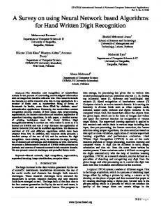
where x r x cos( ) y sin( ) and y r x sin( ) y cos( ) x and y are the spatial dimensions. The Gabor filter is a complex sinusoidal plane wave modulated by a Gaussian envelope, the frequency of which can be varied by the parameter f. and set the standard deviations of the Gaussian envelope along the two spatial dimensions. Angle controls the orientation of the filter. Figure 1 shows the real part of a Gabor filter.
Specific literature on ear tragus extraction using an automated paradigm has not been encountered during the literature review, so the results obtained would provide estimates of detection rates corresponding to a craniofacial landmark not tested earlier. On the other hand, the results obtained with the eye corners can be compared with other researchers’ works. The type of neural network used is a Polynomial Neural Network (PNN). The discriminatory power of a PNN for classification problems has been shown by Huang et al. [19, 28, 41] for face detection, where it was described to have a better performance than a MultiLayer Perceptron (MLP). PNN has been successfully applied for the recognition of handwritten character [42]. PNN combines the input vector by finding product combinations between the input vector elements [43]. The concomitant increase in the dimensionality of the feature space can be reduced by Principal Component Analysis (PCA). For the results presented, the area of interest (AOI) for the different features have been set manually. Automated methods to determine these AOIs can be developed based on gradient and colour information.
Figure 1: Example of Real part of Gabor filter
With the flexibility of the Gabor filter to sweep a wide range of orientations, 8 orientations are normally chosen to cover a full revolution and 5 scales to vary the frequency. The scales are normally chosen to be multiples of 2 so as to keep the frequency bandwidth to 1 octave. So it is a common practice in Machine Vision applications to use 40 masks for feature extraction. The frequencies and orientations are then given by:
2 CRANIOFACIAL LANDMARK EXTRACTION
f max , k 1,2,...,5 2 k 1 (m 1) * 2 m , m 1,2,...,8 8
This section describes the methodology adopted to localise the eye corners and ear tragus given an AOI in which these features are found. The design of the Gabor filter set is described first, followed by its application for extracting the craniofacial landmarks.
fk
(2) (3)
The 2-D Gabor representation in the frequency domain can be formulated as follows:
2.1 Gabor Filter Set Design
2
(u , v , f , ) e
The Gabor filter was first proposed by Dennis Gabor in 1946 [44, 45] to provide a basis for synthesising signals in the time and frequency domain simultaneously. This has been known to involve uncertainty and the Gabor filter has been shown to provide the minimum uncertainty in this respect. Gabor filters have since been used as a feature extraction tool in addition to its original application for signal synthesis. The 2D-Gabor filter can be represented in the normalised form as proposed in [46]: f2
2
f2
f2
( 2 *( ur f ) 2 2 *vr 2 )
(4)
where u r u cos v sin and v r u sin v cos The time and frequency representations clearly show the correspondence of high frequency to a sharper Gaussian envelope and lower frequencies to a broader Gaussian envelope. For a given mask size, it is desirable to choose the filter parameters so that the Gaussian envelope covers the space grid adequately; a coverage of up to two standard (1) be used as a rule of deviations in the two dimensions can thumb to ensure adequate coverage. Clipping the Gaussian envelope before it reaches a low value gives rise to the ‘ringing effect’ in the frequency domain. Another
2
( 2 xr 2 yr ) f2 ( x, y , f , ) *e * e j 2 f xr (1)
15
M. Gooroochurn et al,, International Journal of Science and Advanced Information Technology, 5 (4), July – August 2016, 14-27 consideration in setting the filter parameters for feature extraction is to use a spatial frequency less than or equal to the Nyquist frequency of 0.5 cycles per pixel. Figure 2 shows the magnitude of Gabor filter set over 5 scales and 8 orientations, where the coverage over two standard deviations are shown with equal spread in the two dimensions (==1). The frequency domain representation of this filter set is shown in Figure 3.
the high end of the frequency range, aliasing may occur due to proximity to the Nyquist frequency. Figure 4 shows the change in the frequency distribution by making the parameters and 0.5 and 2 respectively. Figure 5 shows that by using a value of 1.35 for and leads to a frequency coverage along the different orientations where the plots just touch each other.
Figure 2: Magnitude of Gabor Kernels over 5 scales and 8 orientations with fmax = 0.5 cycles per pixel, ==1
Figure 3: Frequency Distribution for fmax = 0.5 cycles per pixel, ==1
The filter design for the feature extraction has a trade-off between dimensionality of the resulting feature set and the maximum operating frequency. On the high end of the mask size, a large feature set leads to a classifier difficult to train and needing a correspondingly large training set, while on
Figure 4: Frequency Distribution for fmax = 0.5 cycles per pixel, (a) ==0.5 (b) ==2
16
M. Gooroochurn et al,, International Journal of Science and Advanced Information Technology, 5 (4), July – August 2016, 14-27 knowing that the information contained in the 31x31 window, to be captured by convolution with a 15x15 kernel, was adequate for representing the landmarks, the filter design strategy adopted has been to use a 15x15 grid size for the Gabor kernels, and to analyse the optimal coverage of a Gaussian envelope in such a way that it reached approximately two standard deviations at the periphery of that 15x15 grid. The final filter set was subsequently derived based on the results of this analysis. A 45 angular spacing has been used as opposed to a 30 spacing due to the lesser number of kernels obtained over the same angle range (0 to 180), which is a critical factor with Polynomial Neural Networks and due to the commonality of using 45 in the Face Processing literature. Figure 6 shows a 15x15 grid with an adjacent Gaussian envelope with standard deviation of 4 pixels so that at the two extremes of the grid in a given dimension, the function reaches a low value (it reaches approximately two standard deviations at the periphery of the 15x15 grid). Figure 5: Frequency Distribution for fmax=0.5 cycles per pixel, ==1.35
The filter set shown in Figure 4(a) is such a case where the frequency bandwidth of the filters at the lowest scale completely encompass the bandwidth of the filters at the other scales. On the other hand, having gaps between the frequency coverage of the different filters leads to poor generalisation of the feature set over untested data. In this case, Figure 4(b) shows a frequency plot that has a sparse coverage and will lead to poor generalisation. By choosing to have equal coverage in the two dimensions, the resultant circular frequency coverage cannot be stacked together without leaving gaps in between, as shown in Figure 5. So in practice, the filter set is designed as a compromise to have some degree of overlap.
Figure 6: 15x15 grid and Gaussian envelope with = 4
Since the same spread is used in the two dimensions, the same Gaussian profile exists in the other dimension, but only one of them is shown in Figure 6. With two scales and an octave separation between the frequencies, this Gaussian envelope would correspond to the smallest frequency and the next higher frequency would be twice this frequency. A 1-D Gaussian function with zero mean has the following form:
The filter set design can be carried out based on the dominant spatial frequencies of the features to be extracted in conjunction with findings obtained from psycho-visual tests. For example, psycho-visual experiments have shown that the Human Visual System has an angular separation of approximately 30 with a frequency separation of an octave [47]. For the filter design task at hand, the aim was to make sure that the spatial coverage of the Gaussian envelope was adequate for the feature window size and the latter was chosen to give a feature space with a low dimensionality. As for the dominant frequency, this cannot be selected for the eye corner and the ear tragus based on spectral analysis as there are likely to be differences among individuals, especially for the ear tragus.
1 g ( z, ) 2
e
z
2
2 2
(5)
Comparing equations (1) and (5),
2 2 2 2 2 and 2 y x 2 2 f f x and y 2f 2f With 1 and x y 4
However, at the scales of the images used, the 31x31 grid size selected for representing the different landmarks (from which the central 15x15 locations are employed to form the feature set) was found consistently to contain adequate information in the neighbourhood of the central location. So
f
17
1 4 2
0.18 and
f max 2 * f 0.36
M. Gooroochurn et al,, International Journal of Science and Advanced Information Technology, 5 (4), July – August 2016, 14-27 Figure 7 shows the two Gaussian envelopes obtained at these two frequencies with equal spread in the two dimensions (==1)
Figure 7: Gaussian Envelopes (a) f = 0.18 cycles per pixel (b) fmax = 0.36 cycles per pixel with ==1 Figure 10: Frequency Distribution with frequencies halved
The corresponding frequency spectrum plotted at 2 standard deviations from the mean is shown in Figure 8. From the frequency plot and the value obtained for fmax (0.36), it is clear that the Nyquist frequency is close. The frequencies of the Gabor filter can be moved away from the Nyquist limiting value of 0.5 by halving the frequency so that f = 0.18 and fmax = 0.09. However making only these changes would expand the Gaussian envelope as the sharpness is formulated in terms of the frequency.
The overlapping of frequency contours at the two frequencies means that the masks obtained by halving the maximum frequency do not contribute to the bandwidth of the filter set. Since it was clear that for such a small grid size as 15x15, a trade-off between Gaussian coverage and maximum usable frequency is inevitable, a maximum frequency of 0.25 per pixel was used with ==1. The resultant Gaussian envelopes and frequency distribution are as shown in Figure 11 and Figure 12 respectively. While the coverage of the Gaussian envelope is adequate for the maximum frequency, the corresponding coverage for a frequency of 0.125 per pixel is not optimal and will lead to ringing effect in the frequency domain. The ringing effect is known to cause blurring at edges when a filter with a sharp cut-off is applied to a image. However, since the aim here is feature extraction rather than image synthesis, a fair degree of ringing due to sharp cut-off can be tolerated although ideally a filter with little ringing would be preferred. Moreover, the ringing effect will have the same effect across the different feature windows collected for training. Since the features obtained are first analysed by PCA, the adverse effect caused by ringing is likely to be suppressed.
Figure 8: Frequency Distribution at two standard deviations
To keep the same sharpness at before, and can be made 0.5 so that effectively, the ratios f/ and f/ do not change. The Gaussian envelopes are shown in Figure 9. As expected, the Gaussian envelopes does not change, but the frequency distribution changes as shown in Figure 10.
Figure 11: Gaussian envelopes for (a) f = 0.125 cycles per pixel (b) fmax = 0.25 cycles per pixel with ==1
Figure 9: Gaussian envelopes with frequencies and normalization factors halved
18
M. Gooroochurn et al,, International Journal of Science and Advanced Information Technology, 5 (4), July – August 2016, 14-27 section describes how these feature vectors were used to train a PNN for locating eye corners. 2.2 Eye Corner Extraction Face images from the AR database [37] were employed for developing the algorithm to extract eye corners in the frontal view. The AR database offers four images for a given subject with variations in lighting. These are: 1. Normal lighting 2. Bright illumination from the left side of the face 3. Bright illumination from the right side of the face 4. Bright illumination over the whole of the face Figure 12: Frequency Distribution for fmax = 0.25 cycles per pixel with ==1
These variations in lighting were used to test the robustness of the algorithm to changes in illumination. One hundred samples of size 31x31, with the outer eye corner located at the centre, were collected from these images. A 1800-element vector was thus generated for each image sample (15x15 central pixels from the 31x31 window over 2 scales and 4 orientations) from the normalised Gabor magnitude response. These samples were used to generate the feature vectors for the true positive training set of the neural network for which outputs of +1 were set.
Due to the lengthy process of validating the suitability of these filter parameters and the mask grid and feature window sizes, a study of any improvement in performance of the classifier over a given training set size has not been carried. It is certainly something worth investigating, e.g. using Gabor mask sizes of 20x20 with 40x40 feature windows, 25x25 mask size with 50x50 feature windows and so forth. The ultimate judge of the suitability of such a filter design paradigm would be the ability of the trained classifier to discriminate between feature and non-feature windows.
Additionally, samples where the outer eye corners were not in the central position of the 31x31 window were collected. Outputs of -1 were set for these samples. A Polynomial Neural Network (PNN) was used as the classifier for the feature detection and localisation. The neural network had one neuron in the output layer and the number of neurons in the input layer was related to the dimensionality of the feature vector. Figure 13 shows the network architecture adopted.
From the response of the Gabor masks over the two scales and four orientations, illumination invariance can be achieved by dividing the responses by the root mean square value of the magnitudes of the responses over all the scales and orientations used. If Gk,m represents the response at scale k and orientation m at a given location (x, y), then the normalisation step for illumination correction can be expressed as follows [21]:
G k' , m
G k ,m
G
(6)
2 k ,m
k ,m
Alternatively, Huang et al. [19] performed illumination correction by subtracting a best-fit intensity plane from the image before applying the Gabor masks. Gabor kernels were generated for frequencies of 0.25 and 0.125 cycles per pixel with unity values for and and orientations of 0, 45, 90 and 135 degrees. These Gabor kernels were convolved with the 31x31 eye corner windows from which the central 15x15 region was selected to form the Gabor feature vector. 8 such 15x15 Gabor response matrices were obtained over the two scales and four orientations applied. The Gabor response, being complex, offers the possibility to use both the phase and magnitude to form the feature vector. However, only the magnitude was used since the feature vector based on both the phase and magnitude led to of high dimensionalities, making it difficult to train the neural networks. The next
Figure 13: PNN Architecture
The overall transformation of the network can be expressed as:
Q T (W * ( z , z.z T ) b) Where T is the activation function, W is the input weight matrix, b is the bias, z is the input vector and from it, the product combinations z.zT is derived. The output of the network is Q. The dimensional expansion in finding product 19
M. Gooroochurn et al,, International Journal of Science and Advanced Information Technology, 5 (4), July – August 2016, 14-27 combinations of the input vector makes it computationally intensive to directly use the 1800 elements of the Gabor feature vector as input since it would increase the number of dimensions to 1800*1800 + 1800. Additionally, having a large dimensionality for the input feature set generally means that the neural network has to be trained over a larger set so as to cover the variation of the input vector sufficiently. This is a necessary condition for neural network solutions to work robustly [14, 22]. So the feature set obtained for the positive samples are first mapped to a lower dimensional basis using (PCA).
been used wherever appropriate. For the case presented above in which 9 was the minimum dimension, 20 dimensions were retained. The dataset is then mapped onto the reduced dimensional space and the product combinations are computed to act as the input for the PNN. Additionally, a further input is computed based on the mapped (z) and original (X) datasets by finding the following distance measure:
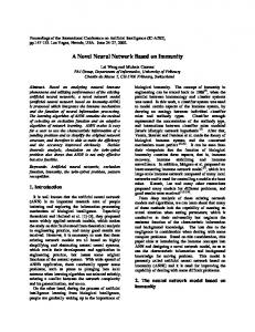
The output of PCA is a set of eigenvectors and eigenvalues, from which the contribution of each eigenvector can be gauged by its corresponding eigenvalue. Although the selection of the number of dimensions to retain in the dataset is arbitrary, the minimum number of dimensions was determined from the eigenvalue spectrum by finding the eigenvalue number at which the sum of eigenvalues arranged in descending order, starting from the smallest and summing towards the largest, equals the largest eigenvalue. This process is illustrated in Figure 14. The feature vector has a dimension of 1800 and thus 1800 eigenvalues are obtained. The largest eigenvalue is found to have a size of about 0.02. The selection of the number of dimensions to be retained starts by summing the eigenvalues’ magnitudes from the 1800th towards the first, and the point where the cumulative sum is equal to the largest eigenvalue is used as an indication of the minimum dimensionality to be retained.
This distance measure is added to the input feature vector. For the example considered earlier where it was decided that 20 dimensions would be retained, this means that the input feature vector to the PNN is 421 (20*20+20+1) instead of 420. The resultant feature set is used to train the PNN. This procedure was followed for extracting the different landmarks.
D ( X X ) 2 z 2
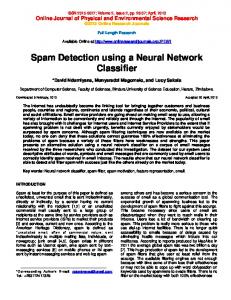
2.2.1 Experimental Results The first test performed was for the outer eye corner for normal and high illumination images. The criterion for successful localisation was set within a 3 pixel margin of the eye corner. The ground truth for the eye corner is based on a subjective inspection. One hundred positive samples taken from four images of twenty-five subjects were collected for the normal and high illumination scenarios. The resultant dataset with a dimensionality of 1800 was analysed by PCA and from the method based on the eigenvalue spectrum described above, 7 dimensions were obtained; so 20 eigenvectors were retained. For subsequent testing, the trained neural network was applied on 300 sample images of subjects not included in the training set, giving a detection rate of 94%. The method of illumination correction used in this case was subtraction of an intensity plane of best-fit. Figure 15 shows some output samples for the outer eye extraction.
Eigenvalue spectrum 0.02 0.018
Eigenvalue magnitude
0.016 0.014 0.012 0.01 0.008 0.006 0.004 0.002 0
0
200
400
600
800 1000 1200 Eigenvalue Number
1400
1600
1800
Figure 14: Example of an Eigenvalue Spectrum
It was found that neural networks trained from product combinations calculated from feature vectors of 20 dimensions (giving about 400 elements) were fast to train and yielded very low mean squared errors, those trained on feature vectors with 25 dimensions (giving about 600 elements) were also relatively easy to train and gave low mean square errors, but neural networks trained on feature vectors with more than 30 dimensions (giving about 900 elements) were more difficult to train. So in subsequent selections of the number of dimensions, 20 and 25 have
Figure 15: Examples of Outer Eye Corners Results [37]
It is worth mentioning that the same tests were run using the intensity values of the central 15x15 pixels as feature 20
M. Gooroochurn et al,, International Journal of Science and Advanced Information Technology, 5 (4), July – August 2016, 14-27 input and a detection rate of 86% was obtained. This confirmed that the Gabor features achieved better results. Moreover, it was evident during testing that the bright images performed poorer compared to normally lit ones, despite their being part of the training set. Thus the next tests performed for the inner eye corner were based only on face samples taken under normal lighting conditions. These amount to two per subjects in the AR database [37] giving fifty samples for training for the same 25 subjects used previously.
whole set of images given in each of these category without any pre-selection. These tests would show the ability to operate in the presence of variations in scale and orientation. The experiment to extract the outer eye corner in the profile view from the FERET database was carried out on a training set containing 100 face images. The feature vectors corresponding to these 100 face images to train the PNN were calculated as described above. From PCA, the minimum number of dimensions required was 24, based on which 25 dimensions were used. The testing of the trained neural network was done on 118 face images not included in the training set, from which a detection rate of 70% was obtained. It was noticed that the neural network was harder to train, especially for the false positives obtained. The training set was augmented with the outer eye corner samples which failed from the 118 profile images. PCA was performed on the new training set, this time a minimum of 29 dimensions was required. So 30 dimensions were retained.
For the tests with the inner eye corner, illumination invariance was achieved by applying Equation (6). A minimum of 9 dimensions was obtained from PCA, based on which 20 dimensions were retained. When tested over 150 subjects not used as part of the training set, 149 successes were recorded. The only case where the algorithm was deemed to have failed was when the PNN response was below 0.5 although the position was correct. Figure 16 shows output samples for inner eye corner extraction.
The increase in the number of dimensions from 25 to 30 correspondingly increased the number of dimensions of the polynomial vector set from 641 (25*25+25+1) to 931 (30*30+30+1). So the resultant network was even harder to train and achieved a mean-square error few orders of magnitudes more than that obtained from tests with the AR database. This is likely to be due to the variation in scale and the size of the neighbourhood captured in the mask being not discriminative enough; it was generally found that the neural network performed badly on the large scale images and either failed due to occlusion of the eye corner by the eyelashes or gave a high net response at the intersection of the eyelashes with the edge of the eyelid, most probably due to the fact that in large scale images, this would appear similar to an eye corner.
Figure 16: Examples of Inner Eye Corner Extraction Results [37]
Since the AR database contains only frontal images, the FERET [38, 39] database was employed to test the same approach for extracting the outer eye corner in the profile and intermediate views. However, the face images given in the FERET database are taken with no control over the scale and it was observed that the angles are not strictly controlled as well. The images given in the FERET database are taken to emulate real-life conditions, and for processing such images using statistical methods, it is common to employ different templates for discrete ranges of angles, and choosing the template that gives the best fit. The scale is normally compensated by using an image pyramid.
The latter problem did not occur for images of smaller scale. Tests on the neural network trained over the augmented set gave a detection rate of 75% when tested over 212 profile images. The marginal improvement in detection rate and the difficulty in training the neural network were factors against the hypothesis that the proposed method can be used at different scales. The neighbourhood size chosen should be adequate to contain enough information about the landmark of interest.
This methodology has not been adopted in extracting the craniofacial features in order to test the performance of the proposed PNN classifier in the presence of such variations. The hypothesis is that the eye corner would appear in the 31x31, although differently and that the PNN would be able to learn these variations. Furthermore, the profile views were mostly correct in orientation and could be adjudged to be so. However, this was harder to do for the 45 degrees intermediate view images. The tests were carried out on the
Tests were also performed on the intermediate 45 degrees views from FERET, where in this case the images have an added variation in that the views were not controlled to be at 45 degrees. So in addition to the variation in scale which was found to deteriorate the network performance, the network was also assessed in its ability to operate with considerable changes in the face orientation. A performance only as good as the previous 75% was expected from these tests. 100 outer eye corner windows were collected and used 21
M. Gooroochurn et al,, International Journal of Science and Advanced Information Technology, 5 (4), July – August 2016, 14-27 to form the training set. PCA yielded a minimum number of 22 dimensions, 25 dimensions were retained.
used as references to the different images to show the variation of the intensity and standard deviation of the images in Figure 18.
The same trend in the neural network being harder to train and leaving a higher mean-square error as compared to that obtained with the AR database was observed. 118 images, not part of the training set, were used to test the detection accuracy, out of which 64% were successful. The training set was augmented with those that failed from the 118 images and the minimum number of dimensions needed was again higher at 28. 30 dimensions were retained to form the input feature set. Upon testing with 240 new images, a detection rate of 67% was obtained. So it can concluded that the variation in rotation also has an adverse effect on the network performance. One face database that uses a camera arrangement with controlled scale and orientation is the CAS-PEAL face database [40]. Part of the CAS-PEAL face database has been made available for research as CAS-PEAL-R1 database. This version of the database was used for performing similar tests as described earlier. With control on the scale and orientation, a better performance was expected. Tests could be performed on the intermediate 45 degrees views only as the profile views of the original database are not included in the current reduced version.
Figure 17: Eye windows processed by gamma manipulation [37]
150 images containing the outer eye corner in the intermediate view were collected and processed with the Gabor masks to generate the feature set. PCA was applied and the minimum number of dimensions obtained from the eigenvalue spectrum method was 15; 20 dimensions were retained. The trained network was tested on 208 face images not used as part of training for which a detection rate of 92% was obtained. The neural networks were easy to train and yielded very low residual error. The detection rate improved to 94% when the false negatives were added to the training set and the trained PNN was tested on 218 images.
2.2.2 Network Tolerance to Illumination Changes and Noise This sections aims to assess the robustness of the proposed feature extraction methodology in general to variations in illumination and random noise. The trained neural network obtained from the AR database is used for this purpose and tested over a single person’s image. The results of this assessment can be applied to correct for brightness in the area of interest, whereas the level of noise at which the network fails gives an indication of its tolerance to typical noise levels encountered in standard camera devices. For testing the performance of the network to illumination changes, gamma manipulation was used to artificially alter the intensity and contrast of the eye window. The set of images obtained are shown in Figure 17 with reference to a for each image. The gamma values are
Figure 18: Variation of Mean Intensity and Standard Deviation with gamma
The range of the mean intensities of the images show that over the gamma values considered, the variation from 22
M. Gooroochurn et al,, International Journal of Science and Advanced Information Technology, 5 (4), July – August 2016, 14-27 normal lighting conditions includes realistic changes. So the result from this analysis can be used to predict the performance of the feature extraction method. It should be noted that that intensity correction by division with the root mean square value of the magnitude of the Gabor response over the scales and orientations used was still applied and the failing of the system was in the presence of such a correction. The trained PNN was tested over these different images. The network did not give any false positives for these images; the network response was zero when it could not detect an eye corner in the image. The network response for the different images, referenced by their gamma values, are shown in Figure 19.
Figure 20: Eye windows corrupted with zero mean Gaussian noise of different standard deviations [37]
Being of random nature, the behaviour of the trained network cannot be gauged on a single degraded image. While it is expected to have a degradation in the network performance with the addition of more Gaussian noise, the behaviour of the network did not show a monotonic degradation in performance. For example, it was found during testing that addition of Gaussian noise at a standard deviation of 0.0009 gave a net response of 0.11 (1 used to signify presence and -1 to signify absence of feature) but a standard deviation of 0.0010 gave a net response of 0.98.
1.4 1.2
Net Response
1 0.8 0.6
A better understanding of the effect of Gaussian noise on the network performance can be obtained by testing over a larger number of images corrupted by Gaussian noise. The results are summarised in a graph in Figure 21, where the network responses with respect to standard deviation of the Gaussian noise over 10 images have been summed up. These tests were carried out on progressively increasing standard deviations until the network was found to give zero values consistently over the most of the ten images.
0.4 0.2 0 -0.2
0
0.5
1
1.5
2
2.5
gamma
Figure 19: Net Response for the different images obtained by gamma manipulation
10
From the variation of the network performance with the changes in image intensity and contrast brought about by gamma manipulations, the range of gamma over which the network performance is satisfactory can be set at 0.55-1.85, assuming a 0.7 threshold is used for the minimum network response for accepting a given pixel as the location for a feature. This corresponds to an intensity range of approximately 60 to 160. So the network is found to tolerate changes in illumination over an acceptable range, and in a well-illuminated environment, it should operate properly.
9 8
Sum of response
7 6 5 4 3 2 1
A common source of noise in image acquisition devices due to the digitisation of the image array and counting of photons on the camera sensor array to yield the intensity of the image can be modelled by Gaussian probability distribution function. Figure 20 shows examples of images obtained for the eye windows when zero mean Gaussian noise was added to varying standard deviations. The standard deviation given for each of the images is normalised to the range [0 1], applied to a normalised greyscale intensity image.
0
0
0.5
1
1.5 Standard Deviation
2
2.5
3 -3
x 10
Figure 21: Variation of network performance with Gaussian noise
It is common practice to perform low pass filtering to reduce Gaussian noise in an image. A similar test methodology was used as described above to assess the performance of the network when a 3x3 equally weighted averaging filter is used prior to the application of the network. The graph in Figure 22 shows the sum of the network performance as a result of applying Gaussian noise 23
M. Gooroochurn et al,, International Journal of Science and Advanced Information Technology, 5 (4), July – August 2016, 14-27 distributions with different standard deviations. From these two graphs (with and without averaging), it is clear that averaging contributes to a better network performance. For example, if a threshold of 0.7 for the network performance is used to accept a location as a feature, then over the 10 images, a value of 7 can be used to decide the point where the performance of the network degrades to unacceptable levels, although from the results obtained, the network behaved in a non-monotonic manner as described before.
2.3 Ear Tragus Extraction The same methodology was adopted for ear tragus extraction as for the eye corner extraction, with the use of the PNN as a classifier and Gabor masks for feature extraction. Normalisation was achieved by dividing by the root mean square magnitude of the Gabor responses. However, during the training set collection, it became evident that the ear structure varies considerably more from subject to subject than the eye corner. The variation occurs in size, shape and complexion of skin. With the variation in the size of the ear structure and due to the fact that the FERET database [38, 39] was used for the initial training and testing where the images have large variations in scale, scaling was applied to make sure the chosen 31x31 window contained the ear tragus, the anti-tragus and the valley linking these two (Figure 23).
10 9 8
Sum of response
7 6 5 4 3 2 1 0
0
0.001 0.002 0.003 0.004 0.005 0.006 0.007 0.008 0.009 Standard Deviation
0.01
Figure 22: Variation of network performance with Gaussian noise and averaging filter
Still for sake of comparison, with averaging, a sum of 7 corresponds to a standard deviation between 0.003 and 0.004 whereas without averaging, it is between 0.001 and 0.0015. Another way to assess the network performance is to look for the range of standard deviations over which all of the ten responses were above 0.7. For the case without averaging, the last standard deviation value at which all the images gave correct localisation and high enough net response (> 0.7) is 0.0007 as the network failed to give any value at one of the images at 0.0008 standard deviation.
Figure 23: General outside ear anatomy and desired ear structure to appear in 31x31 window [38, 39]
Scales of 1, 0.9, 0.8, 0.7 and 0.6 were used during collection of the training set; for a given image, the 31x31 window containing the desired ear structures was saved as a training sample. Samples where this structure did not appear were also collected and used as true negatives in the training set. On the other hand, tests on the CAS-PEAL database [40] did not necessitate any scaling to fit the ear structure inside the 31x31 region as described later.
On the other hand, with averaging, the last standard deviation at which the responses for all the ten images are correct is 0.0012, with a value of 0.46 obtained for one of the images at 0.0014 standard deviation. Since averaging is found to have a definite improvement in the network performance, it can be effectively applied as a preprocessing step. Furthermore, based on a visual inspection of the images shown in Figure 20, the levels of Gaussian noise at which the performance of the network with averaging experiences significant degradation will not be encountered in practice with a camera of reasonable quality, so the performance of the network in the presence of Gaussian noise can be validated to be satisfactory.
2.3.1 Experimental Results The first training was done on 100 profile images from the FERET database [38, 39], followed by tests on 90 samples not used during training. A detection rate of 76% was achieved under a similar criterion of 3 pixels margin from the reference position. The false negative samples were collected and added to the training set for the next training phase. The PNN was trained on the new training set and the false positives collected during subsequent testing. The trained neural network was tested over 181 face samples not used for training, out of which 169 were successful (93% detection rate). The improvement in detection rate can be 24
M. Gooroochurn et al,, International Journal of Science and Advanced Information Technology, 5 (4), July – August 2016, 14-27 attributed to the inclusion of more shape variations of the ear in the training samples. Further inclusion of false negatives and training over more samples is expected to further improve the accuracy. Figure 24 shows output samples for the ear tragus extraction.
from these 81 images were used in the next training phase to augment the training set. With 19 dimensions obtained as the minimum to use, 25 dimensions were again retained. Testing was then done on mirrored images from the Right 45 degrees category. Out of 150 images, 122 gave satisfactory results, representing a detection rate of 82%. So compared to the results obtained with the outer eye corner extraction in the intermediate view, the better performance can be attributed to the compensation for scaling, but the lower performance as compared to extraction from the profile view can be explained by the changes in rotation involved. As pointed out earlier, the CAS-PEAL face database uses a camera arrangement where rotation and scale can be adequately constrained. 150 images were used to collect ear tragus windows without any scaling applied since the desired ear structure were contained in the 31x31 window sizes. PCA was applied on the magnitude of the Gabor response obtained over the same number of scales and orientations. The minimum number of dimensions required was 17; 20 dimensions were retained. The trained network was tested on 156 face images not used as part of training for which a detection rate of 99% was obtained. This again shows the ability of the chosen approach to localise the desired landmarks for adequately constrained scale and rotation images.
Figure 24: Examples of Ear Tragus Extraction Results [38, 39]
The highest response over the different scales was chosen to be the one defining the location of the ear tragus. The performance of the network for images used from the FERET database is likely to be hampered due to the large changes in the scale of the images. Compared to the performance of the PNN-Gabor features method on outer eye corner extraction on the same images from the FERET database, it can be concluded that the use of different scales definitely improved the performance of the network, and as pointed out earlier, the profile images were close to the correct orientation, so scaling helped to make the network invariant to scale changes.
3 DISCUSSION AND CONCLUSION The general theme of this paper has been the testing of a Polynomial Neural Network (PNN) classifier with Gabor features as input vector for the extraction of the ear tragus and eye corners. The tests performed in the presence of illumination variations showed the importance of having images occupying a dynamic range with no significant number of pixels having intensity values close to saturation or black level clipping. Having a normally lit image gives the possibility to use image enhancement techniques to correct for a dark or bright image for improving the network performance. For example, the intensity range obtained from the assessment of the network tolerance to illumination variation was 60 to 160. Gamma correction can thus be applied to shift the intensity distribution of the image so that the mean intensity lies between 60 and 160. Tests with this algorithm has shown an improvement in performance.
The results obtained from the FERET database on intermediate 45 degrees views are presented next. As mentioned earlier, choosing images from the FERET database that are taken close to or at 45 degrees proved to be much harder than for the frontal or profile view. The ear tragus extraction has been done over several scales, so the resultant degradation would be mainly due to rotation. The initial training set was built from 100 face images given in the intermediate view termed as the Left 45 degrees category in the FERET database. A similar procedure was used to generate the Gabor feature vector consisting of 1800 element for each image, and from the 100 samples, the resulting feature space was analysed by PCA. From the eigenvalue spectrum, the minimum number of dimensions found was 17; 25 dimensions were selected to form the basis of the reduced feature space. The trained PNN was tested with the remaining 81 images in that category in which the ear was not occluded by hair. 59 of these gave a positive detection, representing about 73% detection rate. The false negatives
The design of the Gabor filter set attempted to balance the trade-off between the size of the feature set and coverage of the filter envelope. Although a coverage of two standard deviations of the Gaussian envelope is ideal to minimise the ‘ringing effect’ due to sharp cut-off, it was seen that with a 15x15 feature window, it placed the maximum spatial frequency in close proximity to the Nyquist frequency of 0.5 per pixel. So a maximum frequency of 0.25 per pixel was chosen, with the next scale having a frequency of 0.125 per 25
M. Gooroochurn et al,, International Journal of Science and Advanced Information Technology, 5 (4), July – August 2016, 14-27 pixel, which meant that some ‘ringing’ was present in the mask for the lower frequency. The use of PCA to reduce the feature set is likely to suppress any detrimental effect caused by the ringing.
[8] H.A. Rowley, S. Baluja and T. Kanade, Neural network-based face detection, Proceedings CVPR'96 IEEE Computer Society Conference on Computer Vision and Pattern Recognition (1996) 203-208.
Based on the results obtained with the proposed PNN classifier for the ear tragus and eye corner extraction in different views, it can be qualified as a powerful feature detector. The detection rates achieved parallels the results obtained for face detection using Gabor features and PNN by Huang et al. [19] where a detection rate of 100% was obtained over 270 images containing a single face with a simple background.
[9] L. Wiskott et al., Face recognition by elastic bunch graph matching, IEEE Trans. Pattern Anal. Mach. Intell. 19 (1997) 775-779 [10] R. Liao and S.Z. Li, Face recognition based on multiple facial features, Proc. of the 4th IEEE Int. Conf. on Automatic Face and Gesture Recognition (2000) 239-244. [11] T. Kanade, Picture processing system by computer complex and recognition of human faces, Doctoral Dissertation, Dept.of Information Science, Kyoto University, Nov 1973
For more complex images consisting of clutter and multiple faces, Huang et al. obtained a detection rate of 86%. Further tests can be performed with larger sizes of the feature window e.g. 20x20, 25x25 in combination with different sized Gabor masks to assess the effect on the performance of the classifier. The results obtained for the eye corner extraction compare favourably with other feature detectors, while the results obtained for the ear tragus extraction represent, to our knowledge, the first of its type.
[12] P. Viola and M. Jones, Rapid Object Detection using a Boosted Cascade of Simple Features, Proceedings of CVPR2001 Computer Vision and Pattern Recognition 1 (2001) 511-518. [13] K. Sobottka and I. Pitas, Looking for faces and facial features in color images, PRIA: Advances in Mathematical Theory and Applications 7 (1997) 124-137.
REFERENCES [14] A.S.S. Mohamed et al, Face detection based on skin color in image by neural networks, ICIAS 2007 International Conference on Intelligent and Advanced Systems (2007) 779-783.
[1] Li Ganhua et al., An Efficient Face Normalization Algorithm Based on Eyes Detection, IEEE/RSJ International Conference on Intelligent Robots and Systems (2006) 3843-3848.
[15] H.P. Graf et al., Multi-modal system for locating heads and faces, Proceedings of the Second International Conference on Automatic Face and Gesture Recognition (1996) 88–93.
[2] A. Ansari and M. Abdel-Mottaleb, Automatic facial feature extraction and 3D face modeling using two orthogonal views with application to 3D face recognition, Pattern Recognit 38 (2005) 2549-2563
[16] J. Yang and A. Waibel, A real-time face tracker, Proceedings of WACV 96 (1996) 142-147.
[3] R. Niese, A. Al-Hamadi and B. Michaelis, A Stereo and Color-based Method for Face Pose Estimation and Facial Feature Extraction, ICPR 2006 18th International Conference on Pattern Recognition vol 1 (2006) 299-302.
[17] D. Chai and K.N. Ngan, Locating facial region of a head-and-shoulders color image, Proc. Third International Conf. Automatic Face and Gesture Recognition (1998) 124129.
[4] L.M. Brown and Tian Ying-Li, Comparative study of coarse head pose estimation, Proceedings on Motion and Video Computing (2002) 125-130.
[18] R.L. Hsu, M. Abdel-Mottaleb, and A.K. Jain, Face detection in color images, IEEE Trans. Pattern Anal. Mach. Intell., (2002) 696-706.
[5] A. Ansari, M. Abdel-Mottaleb and M.H. Mahoor, 3D Face Mesh Modeling from Range Images for 3D Face Recognition, ICIP 2007 IEEE International Conference on Image Processing 4 (2007) 509-512.
[19] L. Huang, A. Shimizu and H. Kobatake, Robust face detection using Gabor filter features, Pattern Recog. Lett. 26 (2005) 1641-1649
[6] M.H. Yang, D.J. Kriegman and N. Ahuja, Detecting faces in images: A survey, IEEE Trans. Pattern Anal. Mach. Intell. 24(1) (2002) 34-58.
[20] L. Huang, A. Shimizu and H. Kobatake, Face detection from cluttered images using Gabor filter features, SICE 2003 Annual Conference 3 (2003) 29993002
[7] K.K. Sung and T. Poggio, Example-based learning for view-based human face detection, IEEE Trans. Pattern Anal. Mach. Intell. 20 (1998) 39-51. 26
M. Gooroochurn et al,, International Journal of Science and Advanced Information Technology, 5 (4), July – August 2016, 14-27 [21] V. Kyrki, J. Kamarainen and H. Kälviäinen, Simple Gabor feature space for invariant object recognition, Pattern Recog. Lett. 25 (2004) 311-318.
[34] B. Bhanu, and H. Chen, Human ear recognition in 3D, Workshop on Multimodal User Authentication 12 (2003) 91-98.
[22] W. Zhao et al., Face recognition: A literature survey, Acm Computing Surveys (CSUR) 35 (2003) pp. 399-458.
[35] K.H. Pun and Y.S. Moon, Recent advances in ear biometrics, Proceedings of the Sixth IEEE International Conference on Automatic Face and Gesture Recognition (2004) 164-169.
[23] L. Gu, S.Z. Li and H.J. Zhang, Learning probabilistic distribution model for multi-view face detection, IEEE Computer Society Conference on Computer Vision and Pattern Recognition 2 (2001) 116
[36] M. Burge and W. Burger, Ear biometrics, Kluwer International Series in Engineering and Computer Science (1999) 273-286.
[24] H. Schneiderman and T. Kanade, Probabilistic modeling of local appearance and spatial relationships for object recognition, IEEE Computer Society Conference on Computer Vision and Pattern Recognition (1998) 45-51.
[37] A.M. Martinez and R. Benavente, The AR face database, CVC Technical report 1998. [38] P.J. Phillips et al., The FERET database and evaluation procedure for face-recognition algorithms, Image Vision Comput. 16 (1998) 295-306
[25] T.F. Cootes et al., Active shape models-their training and application, Comput. Vision Image Understanding 61 (1995) 38-59.
[39] P.J. Phillips et al., The FERET evaluation methodology for face-recognition algorithms, IEEE Trans. Pattern Anal. Mach. Intell. 22 (2000) 1090-1104.
[26] T.F. Cootes et al., View-based active appearance models, Image Vision Comput. 20 (2002) 657-664. [27] T.F. Cootes, G.J. Edwards and C.J. Taylor, Active appearance models, IEEE Trans. Pattern Anal. Mach. Intell. 23 (2001) 681-685.
[40] W. Gao et al., The CAS-PEAL large-scale Chinese face database and evaluation protocols, Technique Report, No.JDL-TR_04_FR_001, Beijing: Joint Research & Development Laboratory, the Chinese Academy of Sciences (2004).
[28] L.L. Huang et al., Face detection from cluttered images using a polynomial neural network, Proceedings of the International Conference on Image Processing 2 (2001) 669-672
[41] L.L. Huang et al., Gradient feature extraction for classification-based face detection, Pattern Recognit 36 (2003) 2501-2511.
[29] P. Viola and M.J. Jones, Robust real-time face detection, International Journal of Computer Vision 57 (2004) 137-154.
[42] U. Kressel and J. Schurmann, Pattern classification techniques based on function approximation, Handbook of Character Recognition and Document Image Analysis (1997) 49-78.
[30] R. Brunelli and T. Poggio, Face recognition: Features versus templates, IEEE Trans. Pattern Anal. Mach. Intell. 15 (1993) 1042-1052 .
[43] J. Schürmann, Pattern classification: a unified view of statistical and neural approaches, John Wiley & Sons, Inc. New York, NY, USA, 1996).
[31] Y. Ryu and S. Oh, Automatic extraction of eye and mouth fields from a face image using eigenfeatures and multilayer perceptrons, Pattern Recognit 34 (2001) 24592466.
[44] P.C.J. Hill, Dennis Gabor - Contributions to Communication Theory & Signal Processing, EUROCON, The International Conference on "Computer as a Tool" (2007) 2632-2637.
[32] B. Moreno, A. Sanchez and J.F. Velez, On the use of outer ear images for personal identification insecurity applications, Proceedings of IEEE 33rd International Carnahan Conference on Security Technology (1999) 469476.
[45] D. Gabor, Theory of Communication, J. Inst. Electr. Engrs. 93 (1946) 429-457 1946 [46] V. Kyrki, Local and global feature extraction for invariant object recognition, Ph.D. thesis Lappeenranta University of Technology (2002)
[33] P. Yan, and K.W. Bowyer, An automatic 3D ear recognition system, Proceedings of the Third International Symposium on 3D Data Processing, Visualization, and Transmission (3DPVT'06) IEEE Computer Society Washington (2006) 326-333.
[47] D.A. Clausi and M. Ed Jernigan, Designing Gabor filters for optimal texture separability, Pattern Recognit 33 (2000) 1835-1849. 27