A Novel Stochastic Decoding of LDPC Codes with Quantitative

A Novel Stochastic Decoding of LDPC Codes with Quantitative Guarantees Nima Noorshams [email protected]

Aravind Iyengar [email protected]

arXiv:1405.6353v1 [cs.IT] 25 May 2014

Qualcomm Research Silicon Valley Santa Clara, CA, USA May 27, 2014 Abstract Low-density parity-check codes, a class of capacity-approaching linear codes, are particularly recognized for their efficient decoding scheme. The decoding scheme, known as the sum-product, is an iterative algorithm consisting of passing messages between variable and check nodes of the factor graph. The sum-product algorithm is fully parallelizable, owing to the fact that all messages can be update concurrently. However, since it requires extensive number of highly interconnected wires, the fully-parallel implementation of the sum-product on chips is exceedingly challenging. Stochastic decoding algorithms, which exchange binary messages, are of great interest for mitigating this challenge and have been the focus of extensive research over the past decade. They significantly reduce the required wiring and computational complexity of the message-passing algorithm. Even though stochastic decoders have been shown extremely effective in practice, the theoretical aspect and understanding of such algorithms remains limited at large. Our main objective in this paper is to address this issue. We first propose a novel algorithm referred to as the Markov based stochastic decoding. Then, we provide concrete quantitative guarantees on its performance for tree-structured as well as general factor graphs. More specifically, we provide upper-bounds on the first and second moments of the error, illustrating that the proposed algorithm is an asymptotically consistent estimate of the sum-product algorithm. We also validate our theoretical predictions with experimental results, showing we achieve comparable performance to other practical stochastic decoders.

1

Introduction

Sparse graph codes, most notably low-density parity-check (LDPC), have been adopted by the latest wireless communication standards [16, 1, 11, 27]. They are known to approach the channel capacity [30, 21, 29, 28]. What makes them even more appealing for practical purposes is their simple decoding scheme [2, 18]. More specifically, LDPC codes are decoded via a message-passing algorithm called the sum-product (SP). It is an iterative algorithm consisting of passing messages between variable and check nodes in the factor graph [2, 18]. The fact that all messages in the SP algorithm can be updated concurrently, makes the fullyparallel implementation—where the factor graph is directly mapped onto the chip—most efficient. However, due to complex and seemingly random connections between check and variable nodes in the factor graph, fully-parallel implementation of the SP is challenging. The wiring complexity has a big impact on the circuit area and power consumption. Also longer, more inter-connected wires can create more parasitic capacitance and limit the clock rate. Various solutions have been suggested by researchers in order to reduce the implementation complexity of the fully-parallel SP algorithm. Analog circuits have been designed for short LDPC codes [14, 36]. Bit serial algorithms, where messages are transmitted serially over single wires, have been proposed [6, 7, 3, 5]. Splitting row-modules by partitioning check 1

node operations has been shown to provide substantial gains in the required area and power efficiency [22, 23]. In another prominent line of work, researchers have proposed various stochastic decoding algorithms [10, 35, 33, 34, 24, 19, 20, 31]. They are all based on stochastic representation of the SP messages. More precisely, messages are encoded via Bernoulli sequences with correct marginal probabilities. As a result, the structure of check and variable nodes are substantially simplified and the wiring complexity is significantly reduced. (Benefits of such decoders are discussed in more details in Section 3.2.) Stochastic message-passing have also been used in other contexts, among which are distributed convex optimization and learning [17, 13], efficient belief propagation algorithms [25, 26], and efficient learning of distributions [32]. Although experimental results have proved stochastic decoding extremely beneficial, to date mathematical understanding of such decoders are very limited and largely missing from the literature. Since the output of stochastic decoders are random by construction, it is natural to ask the following questions: how does the stochastic decoder behave on average? can it be tuned to approach the performance of SP and if so how fast? is the average performance typical or do we have a measure of concentration around average? The main contribution of this paper is answering these questions by providing theoretical analysis for stochastic decoders. To that end, we propose a novel algorithm, referred to as Markov based stochastic decoding (MbSD), which is amenable to theoretical analysis. We provide quantitative bounds on the first and second moments of the error in terms of the underlying parameters for treestructured (cycle free) as well as general factor graphs, showing that the performance of MbSD converges to that of SP. The remainder of this paper is organized as follows. We begin in Section 2 with some background on factor graph representation of LDPC codes, the sum-product algorithm, and stochastic decoding. In Section 3, we turn to our main results by introducing the MbSD algorithm followed by some discussion on its hardware implementation and statements of our main theoretical results (Theorems 1, and 2). Section 4 is devoted to proofs, with some technical aspects deferred to appendices. Finally in Section 5, we provide some experimental results, confirming our theoretical predictions.

2

Background and Problem Setup

In this section, we setup the problem and provide the necessary background.

2.1

Factor Graph Representation of LDPC Codes

A low-density parity-check code is a linear error-correcting code, satisfying a number of parity check constraints. These constraints are encoded by a sparse parity-check matrix H P t0, 1umˆn . More specifically, a binary sequence x P t0, 1un is a valid codeword if and only 2

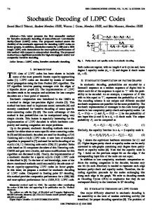
if Hx ” 0, where all operations are module two [30]. A popular approach for modeling LDPC codes is via the notion of factor graphs [18]. A factor graph representing an LDPC code with the parity-check matrix H is a bipartite graph G “ pV, C, Eq, consisting of a set of variable nodes V :“ t1, 2, . . . , nu, a set of check nodes C :“ t1, 2, . . . , mu, and a set of edges connecting variable and check nodes E :“ tpi, aq | i P V, a P C, and Hpa, iq “ 1u. (In this paper, we use letters i, j, . . ., and a, b, . . . to denote variable and check nodes respectively.) A typical factor graph representing an LDPC code (the Hamming code) is illustrated in Figure 1.

2

Figure 1. Factor graph of the Hamming code. Variable nodes are represented by circles, whereas check nodes are represented by squares.

2.2

The Sum-Product Algorithm

Suppose a transmitter sends the codeword x to a receiver over a memory-less, noisy communication channel. Some channel models that are commonly used in practice include the additive white Gaussian noise (AWGN), the binary symmetric channel, and the binary erasure channel. Having received the impaired signal y, the receiver attempts to recover the original signal by finding either the global maximum aposteriori (MAP) estimate x p “ arg maxHx“0 Ppx | yq, or the bit-wise MAP estimates x pi “ arg maxHx“0 Ppxi | yq, for i “ 1, 2, . . . , n. Without exploiting the underlying structure of the code, or equivalently its factor graph, the MAP estimation is intractable and requires an exponential number of operations in the code length. However, this problem can be circumvented using an algorithm called the sumproduct (SP), also known as the belief propagation algorithm. The SP is an iterative algorithm consisting of passing messages, in the form of probability distributions, between nodes of the factor graph [2, 18]. It is known to converge to the correct bit-wise MAP estimates for cycle-free factor graphs; however, on loopy graphs, which includes almost all practical LDPC codes, such a guarantee no longer exists. Nonetheless, the SP algorithm has been shown to be extremely accurate and effective in practice [21, 30]. We now turn to the description of the SP algorithm. For every variable node i P V let N piq :“ ta | pi, aq P Eu denote the set of its neighboring check nodes. Similarly define N paq :“ ti | pi, aq P Eu, the set of neighboring variable nodes for every check node a P C. The SP algorithm allocates two messages to every edge pi, aq P E, one for each direction. At each iteration t “ 0, 1, . . ., every variable node i P V (check node a P C), calculates a message t`1 0 ă αt`1 iÑa ă 1 (message 0 ă αaÑi ă 1) and transmit it to its neighboring check node a P N piq (variable node i P N paq). In updating the messages, every variable node takes into account the incoming messages from its neighboring check nodes as well as the information from the channel, namely αi :“ Ppxi “ 1 | yi q. With this notation at hand, the description of the SP algorithm is as follows: initialize messages from variable to check nodes, α0iÑa “ αi , and update messages for each edge pi, aq P E and iteration t “ 0, 1, . . . according to αtaÑi “

1 1 ´ 2 2

ź

p1 ´ 2 αtjÑaq,

(1)

jPN paqztiu

and αt`1 iÑa “

αi

ś

αi bPN piqztau

ś

bPN piqztau

αtbÑi ` p1 ´ αi q

αtbÑi ś

bPN piqztau p1

´ αtbÑi q

.

(2)

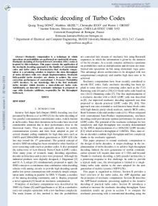
Information flow on a factor graph is shown in Figure 2. Upon receiving all the incoming 3

a

i

j1

a

j2

j3

b

i

(a)

(b)

Figure 2. Graphical representation of message-passing on factor graphs (a) check to variable node (b) variable to check node.

messages, variable node i P V update its marginal probability ś αi bPN piq αtbÑi t`1 ś ś µi “ . αi bPN piq αtbÑi ` p1 ´ αi q bPN piq p1 ´ αtbÑi q

Accordingly, the receiver estimates the i-th bit by x pt`1 “ Ipµt`1 ą 0.5q, where Ip¨q is the i i indicator function. It should also be mentioned that in practice, in order to reduce the quantization error, log-likelihood ratios are mostly used as messages. Moreover, to further simplify the SP algorithm, the check node operation (1) is approximated. The resultant is known as the Min-Sum algorithm [8].

2.3

Stochastic Decoding of LDPC Codes

Stochastic computation in the context of LDPC decoding was first introduced in 2003 by Gaudet and Rapley [10]. Ever since, much research has been conducted in this field and numerous stochastic decoders have been proposed [35, 33, 34, 24, 20, 31]. For instance, Tehrani et al. [33] introduced and exploited the notions of edge memory and noise dependent scaling in order to make the stochastic decoding a viable method for long, practical, LDPC codes. Estimating the probability distributions via a successive relaxation method, LeducePrimeau et al. [20] proposed a scheme with improved decoding gain. More recently, Sarkis et al. [31] extended the stochastic decoding to the case of non-binary LDPC codes. The underlying structure of all these methods and most relevant to our work, however, are the following: they all encode messages by Bernoulli sequences, they all consist of ‘decoding cycles’ which should not be confused with SP iterations (roughly speaking, multiple decoding cycles correspond to one SP iteration.), the check node operation is the module-two sum (i.e. the message transmitted from a check node to a variable node is equal to the module-two sum of the incoming bits.), and finally the variable node operation is the equality (i.e. the message transmitted from a variable node to a check node is equal to one if all incoming bits are one, it is equal to zero if all incoming bits are zero, and it is equal to the previous decoding cycle’s bit in case incoming messages do not agree.). The intuition behind the stochastic variable and check node operations can be obtained from the inspection of SP message updates (1) and (2). More specifically, suppose ZjÑa, for j P N paqztiu, are independent Bernoulli random variables with distributions PpZjÑa “ 1q “ αtjÑa . Then αtaÑi , derived from equation (1), becomes the probability of having odd number of ones in the sequence tZjÑa ujPN paqztiu (see Lemma 1 4

in the paper [9]). Therefore, the statistically consistent estimate of the check to variable node message is the module-two summation of the incoming bits. Similarly, to understand the stochastic variable node operation, let Zi and ZbÑi , for b P N piqztau, be independent Bernoulli random variables with probability distributions PpZi “ 1q “ αi , and PpZbÑi “ 1q “ αtbÑi . Then αt`1 iÑa , derived from equation (2), becomes the probability of the event tZi “ 1, ZbÑi “ 1, @b P N piqztauu, conditioned on the event tZi “ ZbÑi , @b P N piqztauu, thus supporting the intuition that one must transmit the common value from variable to check nodes in case all incoming bits are equal.

3

Algorithm and Main Results

In this section, we introduce the MbSD algorithm, discuss its hardware design aspect, and state some theoretical guarantees regarding its performance.

3.1

The Proposed Stochastic Algorithm

The MbSD algorithm consists of passing messages between variable and check nodes of the factor graph. These messages are 2k-dimensional binary vectors, for a fixed k (design parameter). However, variable and check node updates are element-wise, bit operations. Before stating the algorithm we need to define some notation. Suppose py1 , y2 , . . . , yn q is the received codeword with the likelihood αi “ Ppxi “ 1|yi q, for i “ 1, 2, . . . , n. Our algorithm, involves messages from the channel to variable nodes at every iteration t “ 0, 1, 2, . . .. More specifically, let Zit P t0, 1u2k be the 2k-dimensional binary message from the channel to the variable node i at time t, with independent and identically distributed (i.i.d.) entries PpZit pℓq “ 1q “ αi ,

for all ℓ “ 1, 2, . . . , 2k.

t Moreover, let ZiÑa P t0, 1u2k denote the 2k-dimensional binary message from the variable t node i to the check node a at time t “ 0, 1, . . .. Similarly, let ZaÑi P t0, 1u2k be the message from the check node a to the variable node i at time t. À We also need to define Å the element-wise, module-two summation operator , as well as the “equality” operator . Suppose X , X , . . . , X are arbitrary 2k-dimensional binary 1 2 d Àd vectors. Then, the vector Y “ i“1 Xi denotes the module-two summation of the vectors tXi udi“1 , if and only if 2

Y pℓq ” X1 pℓq ` X2 pℓq ` . . . ` Xd pℓq, Å for all ℓ “ 1, 2, . . . , 2k. Furthermore, by Y “ di“1 Xi we mean $ if Xi pℓq “ 1, for all i “ 1, 2, . . . , d & 1 Y pℓq “ 0 if Xi pℓq “ 0, for all i “ 1, 2, . . . , d % Y pℓ ´ 1q otherwise

,

for all ℓ “ 1, 2, . . . , 2k. Here, we assume Y p0q is either zero or one, equally likely. Now, the precise description of the MbSD algorithm is as follows: 0 1. Initialize messages from variable nodes to check nodes at time t “ 0 by ZiÑa “ Zi0 .

5

(3)

2. For iterations t “ 0, 1, 2, . . ., and every edge pi, aq P E: a) Update messages from check nodes to variable nodes à t t ZaÑi “ ZjÑa . jPN paqztiu

b) Update messages from variable nodes to check nodes by following these steps: – compute the auxiliary variable å

t`1 WiÑa “

t ZbÑi

bPN piqztau

å

Zit`1 .

t`1 – update the message entries ZiÑa pℓq, for ℓ “ 1, 2, . . . , 2k, by drawing i.i.d. samples from the set t`1 t`1 t`1 tWiÑa pk ` 1q, WiÑa pk ` 2q, . . . , WiÑa p2kqu.

c) Compute the binary vector Uit`1 “ estimates according to

Å

aPN piq

ηˆit`1 “

1 k

2k ÿ

t ZaÑi

Å

Zit`1 and update the marginal

Uit`1 pℓq,

(4)

ℓ“k`1

for all i “ 1, 2, . . . , n. Few comments, regarding the interpretation of the algorithm, are worth mentioning at this point. The check to variable node message update (step (a)) is a statistically consistent estimate of the actual check to variable BP message update. However, same can not be stated about the variable Å to check node update (step (b)). As will be shown in Section 4, the equality operator generates Markov chains with desirable properties, thereby, justifying the “Markov based stochastic decoding” terminology. More specifically, the sequence t`1 tWiÑa pℓqu2k ℓ“1 is a Markov chain with the actual variable to check BP message as its stationary distribution. Our objective in step (b) is to estimate this stationary distribution. From basic Markov chain theory, we know that the marginal distribution of a chain converges to its stationary distribution. Therefore, for large enough k, the empirical distribution of the t`1 t`1 t`1 set tWiÑa pk ` 1q, WiÑa pk ` 2q, . . . , WiÑa p2kqu becomes an accurate enough estimate of the t`1 stationary distribution of the Markov chain tWiÑa pℓqu2k ℓ“1 .

3.2

Discussion on Hardware Implementation

The proposed decoding scheme enjoys all the benefits of traditional stochastic decoders [10, 33]. Since messages between variable and check nodes are binary, stochastic decoding requires a substantially lower wiring complexity compared to fully-parallel sum-product or min-sum implementations. Shorter wires yield smaller circuit area, and smaller parasitic capacitance which in turn lead to higher clock frequencies and less power consumption. Another advantage of stochastic decoding algorithms is the very simple structure of check and variable nodes. As a matter of fact, check nodes can be carried out with simple XOR gates, and variable nodes can be implemented using a combination of a random number generator, a JK flip flop, and AND gates [10]. Finally, a very beneficial property of stochastic decoding is the 6

fact that the check node operation (XOR) is associative, i.e., can be partitioned arbitrarily without introducing any additional error. Mohsenin et al. [23], illustrated that partitioning check nodes can provide significant improvements (by a factor of four) in area, throughput, and energy efficiency. It should be noted that in this paper and for mathematical convenience, the messages between check and variable nodes are represented by binary vectors. However, to implement the MbSD algorithm, there is no need to buffer all these vectors. We only need to count the number of ones between bits k ` 1, and 2k in each bulk, which can be accomplished by a simple counter. In that respect, MbSD has a great advantage compared to the algorithm proposed by Tehrani et al. [33], which requires buffering a substantial number of bits on each edge (edge memories). As will be discussed in Section 5, our algorithm has a superior bit error rate performance compared to [33], while maintaining the same order of maximum number of clocks, thereby achieving comparable if not better throughput. Moreover, MbSD is equipped with concrete theoretical guarantees, the subject to which we now turn.

3.3

Main Theoretical Results

Our results concern both cases of tree-structured (cycle free) as well as general factor graphs. Since factor graphs of randomly generated LDPC codes are locally tree-like [30], understanding the behavior of every decoding algorithm (stochastic as well as deterministic) on trees is of paramount importance. To that end, we first state some quantitative guarantees regarding the performance of the proposed stochastic decoder on tree-structured factor graphs. Recalling the fact that there exists a unique path between every two variable nodes in a tree, we denote the largest path (also known as the graph diameter) by L. Moreover, we know that estimates generated by the SP algorithm on a tree converge to true marginals after L iterations [2], i.e., denoting true marginals by tµ˚i uni“1 , we have µti “ µ˚i , for all i “ 1, 2, . . . , n, and t ě L. Theorem 1 (Trees). Consider the sequence of marginals tˆ ηit`1 u8 t“0 , i “ 1, 2, . . . , n, generated by the MbSD algorithm on a tree-structured factor graph. Then for arbitrarily small but fixed parameter δ, and sufficiently large k “ kpδ, Gq we have: (a) The expected stochastic marginals become arbitrarily close to the true marginals, i.e., ˇ “ ‰ ˇ max ˇE ηˆit ´ µ˚i ˇ ď δ, 1ďiďn

for all t ě L.

(b) Furthermore, we have ` ˘ max max var ηˆit “ O

1ďiďn

tě0

ˆ ˙ 1 . k

Remarks: Theorem 1 provides quantitative bounds on the first and second moments of the MbSD marginal estimates. Combining parts (a), and (b), it can be easily observed that ˇ “ ‰ ˇ2 “ t ‰ ` ˘ max E pˆ ηi ´ µ˚i q2 ď max ˇE ηˆit ´ µ˚i ˇ ` max var ηˆit 1ďiďn 1ďiďn 1ďiďn ˆ ˙ 1 , ď δ2 ` O k 7

(5)

for all t ě L. Therefore, as k Ñ 8 (δ Ñ 0), the sequence of estimates ηˆiL (ranging over k) converges to the true marginal µ˚i in the L2 sense. The rate of convergence, and its dependence on the underlying parameters, is fully characterized in expression (17). It is directly a function of the accuracy, and the factor graph structure (diameter, node degrees, etc.), and indirectly (through Lipschitz constants, etc.) a function of the signal to noise ratio (SNR). We now turn to the statement of results for LDPC codes with general (loopy) factor graphs. Unlike tree-structured graphs, the existence and uniqueness of the SP fixed points on general graphs is not guaranteed, nor is the convergence of SP algorithm to such fixed points. Therefore, we have to make the assumption that the LDPC code of interest is well behaved. More precisely, we make the following assumptions: Assumption 1. Suppose the SP message updates are consistent, that is αtiÑa Ñ α˚iÑa , and αtaÑi Ñ α˚aÑi as t Ñ 8 for all directed edges pi Ñ aq, and pa Ñ iq. Equivalently, there exists a sequence tµ˚i uni“1 such that µti Ñ µ˚i , for all i “ 1, 2, . . . , n. For an accuracy parameter δ ą 0, arbitrarily small, we define the stopping time ( T “ T pδq :“ inf t | max |µti ´ µ˚i | ď δ . 1ďiďn

(6)

According to assumption 1, the stopping time T is always finite.

Theorem 2 (General factor graphs). Consider the marginals tˆ ηit`1 u8 t“0 generated by the MbSD algorithm on an LDPC code that satisfies Assumption 1. Then for arbitrarily small but fixed parameter δ, and sufficiently large k “ kpδ, T, Gq we have: (a) The expected stochastic marginals become arbitrarily close to the SP marginals, i.e., ˇ “ t‰ ˇ ˇE ηˆ ´ µt ˇ ď δ, i i for all i “ 1, 2, . . . , n, and t “ 0, 1, . . . , T .

(b) Furthermore, we have ` ˘ max max var ηˆit “ O

1ďiďn 0ďtďT

ˆ ˙ 1 . k

Remarks: Theorem 2, in contrast to Theorem 1, provides quantitative bounds on the error over a finite horizon specified by the stopping time (6). After T “ T pδq iterations, the marginal estimates become arbitrarily close to the true marginals on average; in particular, we have “ ‰ “ ‰ max |E ηˆiT ´ µ˚i | ď max |E ηˆiT ´ µTi | ` max |µTi ´ µ˚i | ď 2 δ. 0ďiďn

0ďiďn

0ďiďn

Moreover, since varpˆ ηiT q “ Op1{kq, as k Ñ 8, the random variables tˆ ηiT uni“1 , become more and more concentrated around their means. Specifically, a very crude bound1 using Chebyshev inequality [12] yields ˆ ˙ ´ n ¯ “ T‰ ` T “ T‰ ˘ T . P max |ˆ ηi ´ E ηˆi | ě ǫ ď n max P |ˆ ηi ´ E ηˆi | ě ǫ “ O 0ďiďn 0ďiďn k ǫ2 Therefore, it is expected that the performance of the proposed stochastic decoding converges to that of SP, as k Ñ 8. 1

Tightening this bound exploiting Chernoff inequality and concentration of measure [4], can be further explored.

8

4

Proof of the Main Results

Conceptually, proofs of Theorems 1 and 2 are very similar. Therefore, in this section, we only prove Theorem 1 and highlight its important differences with Theorem 2 in Appendix D. Poofs make use of basic probability and Markov chain theory. At a high level, the argument consists of two parts: characterizing the expected messages and controlling the error propagationÀ in the factor graph. As it turns out, the check node operations (module two summation ) are consistent on average, that is expected messages from check to variable nodesÅare the same as SP messages. In contrast, the variable node operations (equality operator ) are asymptotically consistent (as k Ñ 8). Therefore, for a finite message dimension k, variable node operations introduce error terms which become propagated throughout the factor graph. The main challenge is to characterize and control these errors.

4.1

Proof of Part paq of Theorem 1

We start by stating Åa lemma which plays a key role in the sequel. Recall the definition of the equality operator from (3).

and Lemma 1. Suppose Zi “ tZi pℓqu8 ℓ“1 , for i “ 1, 2, . . . , d, are stationary, independent, śd identically distributed binary sequence with PpZi pℓq “ 1q “ βi . Then assuming i“1 βi ` Åd śd i“1 Zi forms a time-reversible Markov chain i“1 p1 ´ βi q ą 0, the binary sequence U “ with the following properties: (a) The transition probabilities are d ź ` ˘ βi , P U pℓq “ 1 | U pℓ ´ 1q “ 0 “

` ˘ P U pℓq “ 0 | U pℓ ´ 1q “ 1 “

i“1 d ź

and

(7)

p1 ´ βi q.

(8)

i“1

(b) The stationary distribution is equal to ` ˘ lim P U pℓq “ 1 “ śd

śd

i“1 βi śd i“1 βi ` i“1 p1

ℓÑ8

´ βi q

.

t The proof of this lemma is straight forward and is deferred to Appendix A. Now let βiÑa “ t t ErZiÑa pℓqs “ PpZiÑa pℓq “ 1q be the expected message from the variable node i to the check t node a. By construction and the fact that the variables tZiÑa pℓqu2k ℓ“1 are i.i.d., the expected t t t t value βiÑa is independent of ℓ. Similarly define βaÑi “ ErZaÑi pℓqs “ PpZaÑi pℓq “ 1q, the expected message from the check node a to variable node i. Taking expectation on both sides of the equation (4), we obtain

“ ‰ 1 E ηˆit`1 “ k

2k ÿ

ℓ“k`1

` ˘ P Uit`1 pℓq “ 1 .

(9)

Therefore, in order to upper-bound the expected marginal Erˆ ηit`1 s, we need to calculate the probabilities PpUit`1 pℓq “ 1q, for ℓ “ k ` 1, k ` 2, . . . , 2k. From Lemma 1, we know that the 9

sequence tUit`1 pℓqu2k ℓ“1 is a Markov chain with the following transition probabilities: ź ź t t βaÑi , and git pβq :“ p1 ´ αi q p1 ´ βaÑi q, fit pβq :“ αi aPN piq

(10)

aPN piq

where fit p¨q, and git p¨q are multivariate functions, taking values in the space r0, 1s|N piq| . Recalling the basic Markov chain theory, we can calculate the probability PpUit`1 pℓq “ 1q in terms of the stationary distribution, the iteration number, and the second eigenvalue2 of the transition matrix [12]. Doing some algebra, we obtain ` ˘ ` ˘ ` ˘ P Uit`1 pℓq “ 1 “ P Uit`1 p0q “ 0 P Uit`1 pℓq “ 1 | Uit`1 p0q “ 0 ` ˘ ` ˘ ` P Uit`1 p0q “ 1 P Uit`1 pℓq “ 1 | Uit`1 p0q “ 1 ” gt pβq P`U t`1 p0q “ 1˘ f t pβq P`U t`1 p0q “ 0˘ ı ` ˘ℓ i i 1 ´ fit pβq ´ git pβq ´ i “ i t t t t fi pβq ` gi pβq fi pβq ` gi pβq t f pβq . (11) ` t i fi pβq ` git pβq Substituting equation (11) into (9), doing some algebra simplifying the expression, and exploiting the facts ` ˘ ` ˘ git pβq P Uit`1 p0q “ 1 ´ fit pβq P Uit`1 p0q “ 0 ď fit pβq ` git pβq

and

fit pβq ` git pβq ď αi ` p1 ´ αi q “ 1

(12)

yields “ ‰ E ηˆit`1 ď

fit pβq t fi pβq ` git pβq

On the other hand, denoting ź αtaÑi fit pαq :“ αi

`

` ˘k`1 1 1 1 ´ fit pβq ´ git pβq . t t k fi pβq ` gi pβq

and git pαq :“ p1 ´ αi q

aPN piq

ź

p1 ´ αtaÑi q,

(13)

aPN piq

by definition we have µt`1 “ i

fit pαq . fit pαq ` git pαq

Since the multivariate function fit p¨q{pfit p¨q ` git p¨qq is Lipschitz, assuming mintfit pαq ` git pαq, fit pβq ` git pβqu ě c˚ , for some positive constant c˚ ą 0, there exists a constant M “ M pc˚ q such that “ ‰ |E ηˆit`1 ´ µt`1 i | ď M

ÿ

t |βaÑi ´ αtaÑi | `

aPN piq

1 p1 ´ c˚ qk`1 . k c˚

(14)

Subsequently, in order to upper-bound the error we need to bound the difference between t expected stochastic messages and SP messages, i.e. |βaÑi ´ αtaÑi |. The following lemma, proved in Appendix B, addresses this problem. It is not hard to see that the second eigenvalue of the transition matrix of the Markov chain tUit`1 pℓqu8 ℓ“0 is equal to p1 ´ fit pβq ´ git pβqq. 2

10

Lemma 2. On a tree-structured factor graph and for sufficiently large k, there exists a fixed positive constant c˚ ă 1 such that ( min fit pαq ` git pαq, fit pβq ` git pβq ě c˚ , (15)

for all t “ 0, 1, 2, . . ., and i “ 1, 2, . . . , n. Furthermore, denoting the maximum check and variable node degrees by dc , and dv , respectively, we have t max |βaÑi ´ αtaÑi | ď

paÑiq

pdc ´ 1qp1 ´ c˚ qk`1 rM pdc ´ 1qpdv ´ 1qsL , k c˚ M pdc ´ 1qpdv ´ 1q ´ 1

(16)

for all t “ 0, 1, 2, . . .. Now substituting inequality (16) into (14), we obtain * " “ ‰ rM pdc ´ 1qpdv ´ 1qsL p1 ´ c˚ qk`1 ` 1 , M pd ´ 1qd max |E ηˆit`1 ´ µt`1 | ď c v i 0ďiďn k c˚ M pdc ´ 1qpdv ´ 1q ´ 1 for all t “ 0, 1, 2, . . .. Therefore, setting " * log δ ´ L logpM pdc ´ 1qpdv ´ 1qq 3 k “ max , ˚ , logp1 ´ c˚ q c

(17)

we obtain “ ‰ max |E ηˆit ´ µti | ď δ,

0ďiďn

for all t “ 0, 1, 2, . . ..

4.2

Proof of Part pbq of Theorem 1

To stramline the exposition, let U pℓq :“ Uit`1 pℓq, for fixed i, and t. As previously stated, the sequence tU pℓqu8 ℓ“1 is a Markov chain with initial state p0 :“ PpU p0q “ 0q, p1 :“ PpU p0q “ 1q, and transition probabilities f :“ fit pβq, and g :“ git pβq; more specifically we have ` ˘ ` ˘ f “ P U pℓq “ 1 | U pℓ ´ 1q “ 0 , and g “ P U pℓq “ 0 | U pℓ ´ 1q “ 1 . Since ErpU pℓq ´ ErU pℓqsq2 s ď 1, in order to upper-bound the variance

2k ˘` ˘‰ ` ˘2 ‰ ˘ 2 ÿ “` 1 ÿ “` E U pℓq ´ ErU pℓqs U pℓ1 q ´ ErU pℓ1 qs , var ηˆit`1 “ 2 E U pℓq ´ ErU pℓqs ` 2 k ℓ“k`1 k ℓ1 ăℓ

we only need to upper-bound the cross-product terms. Doing so, for ℓ ą ℓ1 , we have “` ˘` ˘‰ “ ‰ “ ‰ “ ‰ E U pℓq ´ ErU pℓqs U pℓ1 q ´ ErU pℓ1 qs “ E U pℓq U pℓ1 q ´ E U pℓq E U pℓ1 q ` ˘“ ` ˘ ` ˘‰ “ P U pℓ1 q “ 1 P U pℓq “ 1|U pℓ1 q “ 1 ´ P U pℓq “ 1 ` ˘ ` ˘ ď P U pℓq “ 1|U pℓ1 q “ 1 ´ P U pℓq “ 1 .

Now, exploiting the Markov property and equation (11), we can further simplify the aforementioned inequality “` ˘` ˘‰ E U pℓq ´ ErU pℓqs U pℓ1 q ´ ErU pℓ1 qs 1 f p0 g p1 g p1 ´ f ´ gqpℓ´ℓ q ` p1 ´ f ´ gqℓ ´ p1 ´ f ´ gqℓ ď f `g f `g f `g (i)

1

ď p1 ´ f ´ gqpℓ´ℓ q , 11

−1

10

Eb/No=1 Eb/No=2 Eb/No=3 Eb/No=4

−2

−2

bit error rate gap

bit error rate

10

−3

10

−4

10

1

SP SD MbSD, k=64 MbSD, k=128 MbSD, k=256 MbSD, k=512 MbSD, k=1024 1.5

10

−3

10

2

2.5 Eb/No (dB)

3

3.5

2

4

3

10

10 message dimension, k

(a)

(b)

Figure 3. Performance of the MbSD algorithm on a (3,6)-LDPC code with n “ 200 variable nodes and m “ 100 check nodes. (a) Bit error rate versus the energy per bit to noise power spectral density (Eb/No) for different decoders, namely, the SP, the SD (stochastic decoding without noise dependent scaling [33]), and the MbSD for different message dimensions k P t64, 128, 256, 512, 1024u. As predicted by the theory, the performance of the MbSD converges to that of SP. Moreover, MbSD does not suffer from error floor, in contrast to the SD algorithm. (b) Bit error rate gap, i.e., the difference between the SP and the MbSD bit error rates, versus the message dimension. The rate of convergence is upper bounded by Op1{kq, manifested as linear curves in the log-log domain plot.

where inequality (i) follows from (12) and the fact that g{pf ` gq ` p0 f {pf ` gq ď 1. According to Lemma 2, for sufficiently large k, we have f `g ě c˚ . Therefore, putting the pieces together doing some algebra, we obtain ` ˘ 2 1 var ηˆit`1 ď ` 2 k k

ÿ

1

p1 ´ c˚ qpℓ´ℓ q

k`1ďℓ1 ăℓď2k

k´1 1 2 ÿ “ ` 2 pk ´ iqp1 ´ c˚ qi k k i“1

ď

k´1 1 2 ÿ 1 ` 2{c˚ ` , p1 ´ c˚ qi ď k k i“1 k

for all i “ 1, 2, . . . , n, and t “ 0, 1, 2, . . ..

5

Experimental Results

To confirm our theoretical predictions, we test the MbSD algorithm on a simple LDPC code. In our experiments, we set the block-length (variable nodes) and number of parity checks (check nodes) to be n “ 200 and m “ 100, respectively. Using Gallager’s construction [30], we first generate a regular (3, 6)-LDPC code, that is, all variable nodes have degree three, whereas all check nodes have degree six. Then, considering a binary pulse-amplitude modulation (BPAM) system over an AWGN channel, we run MbSD, for t “ 60 iterations, on several simulated signals in order to compute the bit error rate for different values of normalized

12

signal to noise ratio.3 The test is carried out for a number of message dimensions k, and results are compared with the SP algorithm and the stochastic decoding (SD) proposed by Tehrani et al. [33] (see Figure 3 (a)).4 As predicted by our theorems, the performance of the MbSD converges to that of SP as k grows. Therefore, in contrast to the SD algorithm, MbSD is an asymptotically consistent estimate of the SP and does not suffer from error floor. The rate of convergence, on the other hand, can be further explored in Figure 3 (b), wherein the bit error rate gap (i.e., the difference between SP and MbSD bit error rates) versus the message dimension is illustrated. As can be observed, the error curves in the log-log domain plot are roughly linear with slope one. This observation is consistent with equation (5), suggesting the upper-bound of Op1{kq for the rate of convergence. To improve upon the seemingly slow rate of convergence, we make use of the notion of noise dependent scaling (NDS). Sensitivity to random switching activities, referred to as ‘latching’, has been observed to be a major challenge in stochastic decoders [35, 33]. To circumvent this issue, the notion of NDS, in which the received log-likelihoods are down-scaled by a factor proportional to the SNR, was proposed and shown to be extremely effective [33]. The MbSD algorithm suffers from the latching problem too, especially for high SNR values. Intuitively, sequences generated by Markov chains (recall Lemma 1) are likely to be the all-one or the allzero sequences when the SNR is sufficiently high. As a consequence, in such cases, the positive constant c˚ , defined in (15), is more likely to be close to zero. The rate of convergence of the expectation, specified in equation (17), is inversely proportional to logp1 ´ c˚ q, therefore, the smaller the c˚ , the slower the rate of convergence. Resolving this issue requires increasing the switching activities of Markov chain, which is accomplished by the NDS. Figure 4, illustrates the bit error rate versus Eb/No for the SP, the SD using NDS, and the MbSD using NDS.5 As is evident, the rate of convergence of the MbSD algorithm, and thus its performance, is significantly improved. Moreover, having the same number of decoding cycles, MbSD outperforms the SD for high SNRs.

6

Conclusion

In this paper, we studied the theoretical aspect of stochastic decoders, a widely studied solution for fully-parallel implementation of LDPC decoding on chips. Generally speaking, encoding messages by binary sequences, stochastic decoders simplify check and node message updates by modulo-two summation and the equality operator, respectively. As it turns out, the check node operation is statistically consistent on average, whereas, the variable node equality operation generates a Markov chain with the desired quantity as its stationary distribution. Therefore, for a finite message dimension k, the stochastic message updates introduce error terms which become propagated in the factor graph. Controlling these errors is the main challenge in the theoretical analysis of stochastic decoders. To formalize these notions, we introduced a novel stochastic algorithm, referred to as the Markov based stochastic decoding, and provided concrete theoretical guarantees on its performance. More precisely, we showed that expected marginals produced by the MbSD become arbitrarily close to marginals generated by the SP algorithm on tree-structured as well as general factor graphs. The rate 3

A BPAM system with transmit power one over an AWGN channel with noise variance σ 2 has the energy per bit to noise power spectral density (Eb/No) of 1{p2Rσ 2 q, where R is the code rate. 4 In simulating the SD algorithm, we used 30000 ‘decoding cycles’ and edge memory of length 25 without noise dependent scaling. 5 In our simulations we set the NDS scaling parameter to be σ 2 , the optimum choice as suggested in the paper [33].

13

−1

10

SP SD w/ NDS MbSD w/ NDS, k=64 MbSD w/ NDS, k=128 MbSD w/ NDS, k=256

−2

bit error rate

10

−3

10

−4

10

−5

10

1

1.5

2

2.5

3 3.5 Eb/No (dB)

4

4.5

5

Figure 4. Effect of the noise dependent scaling (NDS) on the performance of the MbSD algorithm. The panel contains several plots illustrating the bit error rate versus the energy per bit to noise power spectral density (Eb/No) for different decoders, namely, the SP, the SD (stochastic decoding with noise dependent scaling [33]), and the MbSD for different message dimensions k P t64, 128, 256u. As expected, NDS has significantly improved the performance of the MbSD. Simulations were conducted on a (3,6)-LDPC code with n “ 200 variable nodes and m “ 100 check nodes.

of convergence is governed by the message dimension, the graph structure, and the Lipschitz constant, formally specified in equation (17). Moreover, we proved that the variance of MbSD marginals are upper-bounded by Op1{kq. These theoretical predictions were also supported by experimental results. We showed that, maintaining the same order of decoding cycles, our algorithm does not suffer from error floor; therefore, it achieves better bit error rate performance compared to other competing methods.

Acknowledgements Authors would like to thank Aman Bahtia for providing the C++ code, simulating sumproduct and stochastic decoding algorithms.

A

Proof of Lemma 1

By definition we have $ if Zi pℓq “ 1, for all i “ 1, 2, . . . , d & 1 0 if Zi pℓq “ 1, for all i “ 1, 2, . . . , d . U pℓq “ % U pℓ ´ 1q otherwise

14

Therefore, given U pℓ ´ 1q “ 0 and regardless of the sequence tU pℓ ´ 2q, . . . , U p0qu, the event tU pℓq “ 1u is equivalent to tZi pℓq “ 1, @ i “ 1, . . . , du. Therefore, we have ` ˘ ` ˘ P U pℓq “ 1 | U pℓ ´ 1q “ 0, U pℓ ´ 2q, . . . “ P Zi pℓq “ 1, @i “ 1, . . . , d, piq

“

d d ź ź ` ˘ βi , P Zi pℓq “ 1 “

a“1

i“1

where equality (i) follows from the i.i.d. nature of the sequence. The exact same argument yields the equation (8). Finally, the stationary distribution can be obtained from the detailed balance condition [12] d d ` ˘ ź ` ˘ź βi . p1 ´ βi q “ lim P Ui pℓq “ 0 lim P Ui pℓq “ 1

ℓÑ8

B

ℓÑ8

i“1

i“1

Proof of Lemma 2

t t Recall binary messages ZaÑi , and ZiÑa from steps 2(a) and 2(b) of the main algorithm. Also t t t t recall the definition of expected messages βaÑi “ PpZaÑi pℓq “ 1q, and βiÑa “ PpZiÑa pℓq “ 1q. From Lemma 1 of the paper [9], we know that t βaÑi “

1 1 ´ 2 2

ź

jPN paqztiu

` ˘ t 1 ´ 2βjÑa .

(18)

On the other hand, by construction we have t`1 βiÑa “

1 k

2k ÿ

ℓ“k`1

` t`1 ˘ P WiÑa pℓq “ 1 ,

Å Å t`1 t`1 t where WiÑa “ Zi . Since, according to Lemma 1, the sequence bPN piqztau ZbÑi t`1 tWiÑa pℓqu forms a Markov chain with transition probabilities ź ź t t t t βbÑi , and giÑa pβq :“ p1 ´ αi q p1 ´ βbÑi q, fiÑa pβq :“ αi bPN piqztau

bPN piqztau

basic Markov chain theory yields t pβq ` t`1 ˘ fiÑa P WiÑa pℓq “ 1 “ t t fiÑa pβq ` giÑa pβq ` ˘ ` t`1 ˘ ” g t pβqP W t`1 p0q “ 1 t ˘ℓ fiÑapβqP WiÑa p0q “ 0 ı ` iÑa iÑa t t ` 1 ´ fiÑa pβq ´ giÑa pβq . ´ t t t t fiÑa pβq ` giÑa pβq fiÑapβq ` giÑa pβq

Therefore, doing some algebra, noticing the facts that ` t`1 ˘ ` t`1 ˘ t t giÑa pβqP WiÑa p0q “ 1 fiÑa pβqP WiÑa p0q “ 0 ´ ď 1 t t t t fiÑa fiÑa pβq ` giÑa pβq ` giÑa pβq pβq and t t fiÑa pβq ` giÑa pβq ď αi ` p1 ´ αi q “ 1,

15

we have t`1 βiÑa ď

t 1 fiÑa pβq t t ` p1 ´ fiÑa pβq ´ giÑa pβqqk`1 . t t t t fiÑapβq ` giÑa pβq k pfiÑa pβq ` giÑa pβqq

(19)

Equations (18), and (19) characterize the stochastic decoding message updates. Similarly, we have the SP update equations for all directed edges αtaÑi “

1 1 ´ 2 2

ź

jPN paqztiu

`

˘ 1 ´ 2αtjÑa ,

and αt`1 iÑa “

t fiÑa pαq , t t fiÑa pαq ` giÑa pαq

(20)

where we have denoted t fiÑa pαq :“ αi

ź

t and giÑa pαq :“ p1 ´ αi q

αtbÑi ,

ź

p1 ´ αtbÑi q.

bPN piqztau

bPN piqztau

t Since 0 ď αtjÑa ď 1, and 0 ď βjÑa ď 1, for all t, and pj Ñ aq, we have6 ÿ t`1 t`1 |βaÑi ´ αt`1 | ď |βjÑa ´ αt`1 aÑi jÑa |.

(21)

jPN paqztiu

We now turn to upper-bounding the term t t ˇ fjÑa pαq fjÑa pβq ˇ ´ ˇ t t t t fjÑapβq ` gjÑa pβq fjÑapαq ` gjÑa pαq 1 t t ` p1 ´ fjÑa pβq ´ gjÑa pβqqk`1 . t t k pfjÑa pβq ` gjÑa pβqq

ˇ ˇ t`1 |βjÑa ´ αt`1 | ď ˇ jÑa

Since 0 ă α0jÑa “ αj ă 1. Then by inspection of the SP updates, it is easy to see that 0 ă αtjÑa ă 1, and 0 ă αtaÑj ă 1, for all t ě 0, and all directed edges pa Ñ jq, and pj Ñ aq. Therefore, recalling the definition (13), and the fact that αtaÑi “ α˚aÑi , for t larger than the graph diameter, there exists a positive constant c˚ ă 1 such that fjt pαq ` gjt pαq ě 2 c˚ ,

j “ 1, 2, . . . , n, and t “ 0, 1, 2, . . . .

for all

Now we show that for sufficiently large k, we have fjt pβq ` gjt pβq ě c˚ ,

for all

Suppose for a fixed t, we have ÿ τ |βaÑj ´ ατaÑj | ď c˚ ,

j “ 1, 2, . . . , n, and t “ 0, 1, 2, . . . .

for all

j “ 1, 2, . . . , n, and τ “ 0, 1, . . . , t.

(22)

(23)

aPN pjq

0 Since βjÑa “ α0jÑa “ αj , the left hand side of the above inequality is initially equal to zero; thus the condition (23) is satisfied for t “ 0. Now making use of the mean-value theorem, we obtain7 ÿ τ |fjτ pβq ` gjτ pβq ´ fjτ pαq ´ gjτ pαq| ď |βaÑj ´ ατaÑj |. aPN pjq

6

The inequality follows from the mean-value theorem and the fact that for the function ś hpx1 , . . . , xd q “ di“1 p1 ´ 2xi q{2, we have |Bh{Bxi | ď 1, if 0 ă xi ď 1 for all i “ 1, . . . , d. śd śd 7 Let hpx1 , . . . , xd q “ α ś i“1 xi ` p1 ´ αq i“1 p1 ´ xi q be an arbitrary function for 0 ď xi ď 1, i “ 1, . . . , d. ś Then we have |Bh{Bxi | ď α j‰i xj ` p1 ´ αq j‰i p1 ´ xj q ď 1.

16

Putting the pieces together, assuming (23), yields fjτ pβq ` gjτ pβq ě c˚

for all

j “ 1, 2, . . . , n, and τ “ 0, 1, . . . , t.

t Since 0 ď βaÑj , αtaÑj ď 1, we have τ τ fjÑa pβq ` gjÑa pβq ě fjτ pβq ` gjτ pβq ě c˚ ,

and

τ τ fjÑa pαq ` gjÑa pαq ě fjτ pαq ` gjτ pαq ě 2 c˚ ;

therefore, there exist a constant M “ M pc˚ q such that τ `1 τ `1 | ď M ´ αjÑa |βjÑa

ÿ

τ |βbÑj ´ ατbÑj | `

bPN pjqztau

1 p1 ´ c˚ qk`1 , k c˚

(24)

for all τ “ 0, 1, . . . , t. Substituting the inequality (24) into (21), we obtain ÿ

τ `1 τ `1 |βaÑi ´ αaÑi | ď M

ÿ

τ ´ ατbÑj | ` |βbÑj

jPN paqztiu bPN pjqztau

pdc ´ 1qp1 ´ c˚ qk`1 , k c˚

(25)

t whereřwe have denoted dc :“ max0ďaďm |N paq|. Let et :“ t|βaÑi ´ αtaÑi |upaÑiq be the m r :“ a“1 |N paq| dimensional error vector. Now define a matrix A P Rrˆr with entries indexed by pairs of directed edges pa Ñ iq; in particular, we have " M if j P N paqztiu and b P N pjqztau Apa Ñ i, b Ñ jq :“ . (26) 0 o.w.

Then by stacking the scalar inequalities (25), we obtain the vector inequality eτ `1 ĺ A eτ `

pdc ´ 1qp1 ´ c˚ qk`1 ~ 1, k c˚

(27)

for all τ “ 0, 1, . . . , t. Here, ĺ denotes the vector inequality, i.e., for r-dimensional vectors x, and y we say x ĺ y if and only if xpiq ď ypiq, for all i “ 1, 2, . . . , r. Unwrapping the recursion (27), noticing that e0 “ ~0, we obtain et`1 ĺ

˘ pdc ´ 1qp1 ´ c˚ qk`1 ` I ` A ` . . . ` At ~1. ˚ kc

(28)

The right hand side sequence of the previous inequality have, seemingly, a growing number of terms as t Ñ 8. However, according to the following lemma, proved in Appendix C, the graph-respecting matrix A is nilpotent, i.e., there exists a positive integer ℓ such that Aℓ “ 0. (A similar statement regarding nilpotence of the tree-structured Markov random field have been shown in Lemma 1 [26].) Recall the definition of the factor graph diameter L, the largest path between any pair of variable nodes. Lemma 3. The graph-respecting matrix A, defined in (26), is nilpotent with degree at most the diameter of the factor graph L, that is AL “ 0. Exploiting the result of Lemma 3, we can further simplify the vector inequality (28) et ĺ

˘ pdc ´ 1qp1 ´ c˚ qk`1 ` I ` A ` . . . ` AL´1 ~1, ˚ kc 17

(29)

for all t “ 0, 1, 2, . . .. Now we take } ¨ }8 on the both sides of the inequality (29). Recalling the definition of the matrix norm infinity8 , ||| ¨ |||8 , triangle inequality, and using the fact that |||Aℓ |||8 ď |||A|||ℓ8 [15], simple algebra yields max

paÑiq

t`1 |βaÑi

´

αt`1 aÑi |

L´1 pdc ´ 1qp1 ´ c˚ qk`1 ÿ |||A|||ℓ8 ď k c˚ ℓ“0

ď

L´1 pdc ´ 1qp1 ´ c˚ qk`1 ÿ rM pdc ´ 1qpdv ´ 1qsℓ k c˚ ℓ“0

ď

pdc ´ 1qp1 ´ c˚ qk`1 rM pdc ´ 1qpdv ´ 1qsL , k c˚ M pdc ´ 1qpdv ´ 1q ´ 1

where we have denoted dv “ max0ďiďn |N piq|. For sufficiently large k, specifically when pdc ´ 1qp1 ´ c˚ qk`1 rM pdc ´ 1qpdv ´ 1qsL c˚ ď , k c˚ M pdc ´ 1qpdv ´ 1q ´ 1 dv we have

ÿ

t`1 ˚ |βaÑj ´ αt`1 aÑj | ď c ,

for all

j “ 1, 2, . . . , n,

aPN pjq

and hence fjt`1 pβq ` gjt`1 pβq ě c˚ , which proves the claim (22) and concludes the lemma.

C

Proof of Lemma 3

We first show, via induction, that for any the entry Aℓ pa Ñ i, b Ñ jq ‰ 0 if and between the edges pb Ñ jq, and pa Ñ iq. non-overlapping, directed (check-variable)

positive integer ℓ and edges pa Ñ iq, and pb Ñ jq, only if there exists a directed path of length9 ℓ More specifically, there must exists a sequence of edges tpa1 Ñ i1 q, . . . , paℓ´1 Ñ iℓ´1 qu such that

b P N pjqztaℓ´1 u, j P N paℓ´1 qztiℓ´1 u, . . . , a1 P N pi1 qztau, i1 P N paqztiu. The base case for ℓ “ 1, is obvious from construction (26). Suppose the claim is correct for ℓ; the goal is to prove it for ℓ ` 1. By definition, we have ÿ Aℓ`1 pa Ñ i, b Ñ jq “ Aℓ pa Ñ i, c Ñ kq Apc Ñ k, b Ñ jq. pcÑkq

Since the matrix is non-negative, Aℓ`1 pa Ñ i, b Ñ jq ‰ 0, if and only if there exists an edge pc Ñ kq such that Aℓ pa Ñ i, c Ñ kq ‰ 0, and Apc Ñ k, b Ñ jq ‰ 0. Therefore, according to the induction hypothesis, there exist a sequence of non-overlapping edges tpa1 Ñ i1 q, . . . , paℓ´1 Ñ iℓ´1 qu such that c P N pkqztaℓ´1 u, k P N paℓ´1 qztiℓ´1 u, . . . , a1 P N pi1 qztau, i1 P N paqztiu. Moreover, we should have b P N pjqztcu, and j P N pcqztku. Putting the pieces together, there must exists a directed path of length ℓ`1, consisting of tpa1 Ñ i1 q, . . . , paℓ´1 Ñ iℓ´1 q, pc Ñ kqu, between edges pb Ñ jq, and pa Ñ iq, which yields the claim. Finally, since there is no directed path longer than L (diameter) between any pair of edges in a tree-structured factor graph, we must have AL “ 0 that concludes the proof. 8 9

Norm infinity of a matrix is the maximum absolute row sum of the matrix [15] Here the length of the path is equal to the number of intermediate variable nodes plus one.

18

D

Proof of Theorem 2

As stated previously, proof of Theorem 2 is similar to that of Theorem 1. The major difference lie in the fact that due to its cycle-free structure, tree-respecting matrix A, defined in (26), is nilpotent (recall the result of Lemma 3). However, the same may not necessarily be true for general graphs. As a consequence, for a non-tree factor graph, the right hand side of the inequality (28) has indeed a growing number of terms as t Ñ 8. However, we can upperbound the error over a finite horizon provided by the stopping time T , defined in (6). More precisely, unwrapping the recursion (27) for τ “ 0, 1, . . . , t, taking norm-infinity on both sides of the outcome, and doing some algebra yields pdc ´ 1qp1 ´ c˚ qk`1 rM pdc ´ 1qpdv ´ 1qst`1 , k c˚ M pdc ´ 1qpdv ´ 1q ´ 1

t`1 max |βaÑi ´ αt`1 aÑi | ď

paÑiq

for all t “ 0, 1, . . . , T ´ 1. Therefore, for k sufficiently large, specifically when pdc ´ 1qp1 ´ c˚ qk`1 rM pdc ´ 1qpdv ´ 1qsT c˚ ď , k c˚ M pdc ´ 1qpdv ´ 1q ´ 1 dv we have ÿ

t`1 ˚ |βaÑj ´ αt`1 aÑj | ď c ,

aPN pjq

for all j “ 1, 2, . . . , n, and t “ 0, 1, . . . , T ´ 1, thereby completing the proof of a slightly different version of the Lemma 2 over a finite horizon. Lemma 4. For sufficiently large k, there exists a fixed positive constant c˚ “ c˚ pT q ă 1 such that ( min fit pαq ` git pαq, fit pβq ` git pβq ě c˚ , for all t “ 0, 1, . . . , T , and i “ 1, 2, . . . , n. Furthermore, we have t max |βaÑi ´ αtaÑi | ď

paÑiq

pdc ´ 1qp1 ´ c˚ qk`1 rM pdc ´ 1qpdv ´ 1qst , k c˚ M pdc ´ 1qpdv ´ 1q ´ 1

(30)

for all t “ 0, 1, . . . , T . Now substituting the inequality (30) into (14), setting " * log δ ´ T logpM pdc ´ 1qpdv ´ 1qq 3 k “ max , ˚ , logp1 ´ c˚ q c we obtain “ ‰ max |E ηˆit ´ µti | ď δ,

0ďiďn

for all t “ 0, 1, . . . , T , which concludes proof of part (a) of Theorem 2. Proof of part (b) follows the exact same steps outlined in the Section 4.2

19

References [1] IEEE 802.16e. Air interface for fixed and mobile broadband wireless access systems, October 2005. IEEE p802.16e/d12 Draft. [2] S. M. Aji and R. J. McEliece. The generalized distributive law. IEEE Transactions on Information Theory, 46(2):325–343, March 2000. [3] Tyler Brandon, Robert Hang, Gary Block, Vincent C. Gaudet, Bruce Cockburn, Sheryl Howard, Christian Giasson, Keith Boyle, Paul Goud, Siavash Sheikh Zeinoddin, Anthony Rapley, Stephen Bates, Duncan Elliott, and Christian Schlegel. A scalable LDPC decoder ASIC architecture with bit-serial message exchange. the VLSI Journal of Integration, 41(3):385 – 398, 2008. [4] F. Chung and L. Lu. Concentration inequalities and martingale inequalities: A survey. Internet Mathematics, 3(1):79–127, 2006. [5] K. Cushon, C. Leroux, S. Hemati, S. Mannor, and W.J. Gross. A min-sum iterative decoder based on pulsewidth message encoding. IEEE Transactions on Circuits and Systems II: Express Briefs, 57(11):893–897, 2010. [6] A. Darabiha, A. C. Carusone, and F. R. Kschischang. A bit-serial approximate minsum ldpc decoder and FPGA implementation. In Proceedings of the IEEE International Symposium on Circuits and Systems, May 2006. [7] A. Darabiha, A. C. Carusone, and F. R. Kschischang. Power reduction techniques for LDPC decoders. IEEE Journal of Solid-State Circuits, 43(8):1835–1845, 2008. [8] M. P. C. Fossorier, M. Mihaljevic, and H. Imai. Reduced complexity iterative decoding of low-density parity check codes based on belief propagation. IEEE Transactions on Communications, 47(5):673–680, May 1999. [9] R. G. Gallager. Low-density parity check codes. IRE Transactions on Information Theory, 8(1):21–28, 1962. [10] V. C. Gaudet and A. C. Rapley. Iterative decoding using stochastic computation. Electronics Letters, 39(3):299–301, 2003. [11] G.hn/G.9960. Next generation http://www.itu.int/ITU-T.

standard

for

wired

home

network.

[12] G. R. Grimmett and D. R. Stirzaker. Probability and Random Processes. Oxford Science Publications, Clarendon Press, Oxford, 1992. [13] E. Hazan, A. Agarwal, and S. Kale. Logarithmic regret algorithms for online convex optimization. Journal of Machine Learning, 69(2-3):169–192, 2007. [14] S. Hemati, A. H. Banihashemi, and C. Plett. A 0.18- µm CMOS analog min-sum iterative decoder for a (32,8) low-density parity-check (LDPC) code. IEEE Journal of Solid-State Circuits, 41(11):2531–2540, 2006. [15] R. A. Horn and C. R. Johnson. Matrix Analysis. Cambridge University Press, Cambridge, 1985. 20

[16] T. T. S. I. Digital video broadcasting (DVB) second generation framing structure for broadband satellite applications. http://www.dvb.org. [17] A. Juditsky, G. Lan, A. Nemirovski, and A. Shapiro. Robust stochastic approximation approach to stochastic programming. SIAM Journal on Optimization, 19(4):1574–1609, 2009. [18] F. R. Kschischang, B. J. Frey, and H. A. Loeliger. Factor graphs and the sum-product algorithm. IEEE Transaction on Information Theory, 47(2):498–519, 2001. [19] H. Kuo-Lun, V. Gaudet, and M. Salehi. A Markov chain model for edge memories in stochastic decoding of ldpc codes. In Proceedings of the 45th Annual Conference on Information Sciences and Systems, pages 1–4, 2011. [20] F. Leduc-Primeau, S. Hemati, S. Mannor, and W. J. Gross. Relaxed half-stochastic belief propagation. IEEE Transactions on Communications, 61(5):1648–1659, 2013. [21] D. MacKay. Good error correcting codes based on very sparse matrices. IEEE Transactions on Information Theory, 45(2):399–431, 1999. [22] T. Mohsenin and B. M. Baas. Split-row: A reduced complexity, high throughput LDPC decoder architecture. In Proceedings of International Conference on Computer Design, pages 320–325, 2006. [23] T. Mohsenin, D. N. Truong, and B. M. Baas. A low-complexity message-passing algorithm for reduced routing congestion in LDPC decoders. IEEE Transactions on Circuits and Systems I: Regular Papers, 57(5):1048–1061, 2010. [24] A. Naderi, S. Mannor, M. Sawan, and W. J. Gross. Delayed stochastic decoding of LDPC codes. IEEE Transactions on Signal Processing, 59(11):5617–5626, 2011. [25] N. Noorshams and M. J. Wainwright. Belief propagation for continuous state spaces: Stochastic message-passing with quantitative guarantees. Journal of Machine Learning Research, 14:2799–2835, September 2013. [26] N. Noorshams and M. J. Wainwright. Stochastic belief propagation: A low-complexity alternative to the sum-product algorithms. IEEE Transactions on Information Theory, 59(4):1981–2000, April 2013. [27] IEEE P802.3an. 10GBASE-T Task forse. http://www.ieee802.org/3/an. [28] T. Richardson, A. Shokrollahi, and R. Urbanke. Design of capacity-approaching irregular low-density parity check codes. IEEE Transactions on Information Theory, 47:619–637, February 2001. [29] T. Richardson and R. Urbanke. The capacity of low-density parity check codes under message-passing decoding. IEEE Transactions on Information Theory, 47:599–618, February 2001. [30] T. Richardson and R. Urbanke. Modern Coding Theory. Cambridge University Press, 2008. [31] G. Sarkis, S. Hemati, S. Mannor, and W. J. Gross. Stochastic decoding of LDPC codes over GF(q). IEEE Transactions on Communications, 61(3):939–950, 2013. 21

[32] A. D. Sarwate and T. Javidi. Opinion dynamics and distributed learning of distributions. In Proceedings of the 49th Annual Allerton Conference on Communication, Control, and Computing, pages 1151–1158, September 2011. [33] S. S. Tehrani, W. J. Gross, and S. Mannor. Stochastic decoding of LDPC codes. IEEE Communications Letters, 10(10):716–718, 2006. [34] S. S. Tehrani, A. Naderi, G. A. Kamendje, S. Hemati, S. Mannor, and W. J. Gross. Majority-based tracking forecast memories for stochastic LDPC decoding. IEEE Transactions on Signal Processing, 58(9):4883–4896, 2010. [35] C. Winstead, V. C. Gaudet, A. Rapley, and C. Schlegel. Stochastic iterative decoders. In Proceedings of the International Symposium on Information Theory, pages 1116–1120, February 2005. [36] C. Winstead, N. Nguyen, V.C. Gaudet, and C. Schlegel. Low-voltage CMOS circuits for analog iterative decoders. IEEE Transactions on Circuits and Systems I: Regular Papers, 53(4):829–841, 2006.

22