Mar 16, 2011 - IT] 15 Mar 2011 .... However, the underlying codes discussed in [15] are based on factor ... Note that similar to [14], the bounds of [15] are.
Reweighted LP Decoding for LDPC Codes Amin Khajehnejad∗ Alexandros G. Dimakis† Babak Hassibi∗ Benjamin Vigoda+ William Bradley+ ∗
California Institute of Technology
†
University of Southern California
arXiv:1103.2837v1 [cs.IT] 15 Mar 2011
+
Lyric Semiconductors Inc.
∗
March 16, 2011
Abstract We introduce a novel algorithm for decoding binary linear codes by linear programming. We build on the LP decoding algorithm of Feldman et al. and introduce a post-processing step that solves a second linear program that reweights the objective function based on the outcome of the original LP decoder output. Our analysis shows that for some LDPC ensembles we can improve the provable threshold guarantees compared to standard LP decoding. We also show significant empirical performance gains for the reweighted LP decoding algorithm with very small additional computational complexity.
1
Introduction
Linear programming (LP) decoding for binary linear codes was introduced by Feldman, Karger and Wainwright [2]. The method is based on solving a linear-programming relaxation of the integer program corresponding to the maximum likelihood (ML) decoding problem. LP decoding is connected to message-passing decoding [3, 4], and graph covers [5, 6] and has received substantial recent attention (see e.g. [6], and [7]). As with the work described here, a related line of work has studied various improvements to either standard iterative decoding [8, 9] or to LP decoding via nonlinear extensions [10] or loop corrections [11]. The practical performance of LP decoding is roughly comparable to min- sum decoding and slightly inferior to sum-product decoding. In contrast to message-passing decoding, however, the ∗ This work was supported in part by the National Science Foundation under grants CCF-0729203, CNS-0932428 and CCF-1018927, by the Office of Naval Research under the MURI grant N00014-08-1-0747, by Caltech’s Lee Center for Advanced Networking and by DARPA FA8750-07-C-0231.
1
LP decoder either concedes failure on a problem, or returns a codeword along with a guarantee that it is the ML codeword, thereby eliminating any undetected decoding errors. The main idea of this paper is to add a second LP as a post-processing step when original LP decoding fails and outputs a fractional pseudocodeword. We use the difference between the input channel likelihood and the pseudocodeword coordinate to find a measure of disagreement or unreliability for each bit. We subsequently use this unreliability to bias the objective function and re-run the LP with the reweighted objective function. The reweighting increases the cost of changing reliable bits and decreases the cost for unreliable bits. We present an analysis that the provable BSC recovery thresholds improve for certain families of LDPC codes. We stress that the actual thresholds, even for the original LP decoding algorithm, remain unknown. Our analysis only establishes that the obtainable lower bounds on the fraction of recoverable errors are improved compared to the corresponding bounds for LP decoding. It is possible, however, that this is just an artifact of the lower bound techniques and that the true threshold is identical for both algorithms. In any case, the empirical performance gains we observe in our preliminary experimental analysis seem quite substantial. A central idea in our analysis is a notion of robustness to changes in the BSC bit-flipping probability. This concept was inspired by a similar reweighted iterative `1 minimization idea for compressive sensing [21, 20]. We note that the reweighting idea of this paper involves changing the objective function of the LP from the reweighted max- product algorithm [12].
2
Basic Definitions
A vector x in Rn is called k-sparse if it has exactly k nonzero entries. The support set of a sparse vector x is the index set of its nonzero entries. If x is not sparse, the k-support set of x is defined as the index set of the maximum k entries of x in magnitude. We use kxkp to denote the `p norm of a vector x for p ≥ 0. in particular kxk0 is defined to be the number of nonzero entries in x. For a set S, cardinality of S is denoted by |S| and if S ⊂ {1, 2, · · · , n}, then xS is the sub-vector formed by those entries of x indexed in S. Also the complement set of S is denoted by S c . The rate of a linear binary code C is denoted by R, and the corresponding parity check matrix is H ∈ Fm×n , where n is the length of each codeword and m = Rn. The factor graph corresponding to C is denoted by G = (Xv , Xc , E), where Xv and Xc are the sets of variable nodes and check nodes respectively, and E is the set of edges. For regular graphs, dv and dc denote the degree of variable and check nodes respectively. The girth of a graph G, denoted by girth(G), is defined to be the size of the smallest cycle in G.
2
3
Background
Suppose that C is a memoryless channel with binary input and an output alphabet Y, defined by the transition probabilities PY |X (y|x). For a received symbol y, the likelihood ratio is defined P
(y|x=0)
as log( PY |X (y|x=1) ), where x is the transmitted symbol. If a codeword x(c) of length n from Y |X
the linear code C is transmitted through the channel, and an output vector x(r) is received, a maximum likelihood decoder can be used to estimate the transmitted codeword by finding the most likely transmitted input codeword. Let γi be the likelihood ratio assigned to the ith (r)
received bit xi , and γ be the likelihood vector γ = (γ1 , · · · , γn )T . The ML decoder can be formalized as follows [1]
ML decoder:
minimize γ T x subject to x ∈ conv(C),
(1)
where conv(C) is the convex hull of all the codewords of C in Rn . The linear program (1) solves the ML decoding problem by the virtue of the fact that the objective γ T x is minimized by a corner point (or vertex) of conv(C), which is necessarily a codeword (In fact, vertices of conv(C) are all the codewords of C). In a linear program, the polytope over which the optimization is performed is described by linear inequalities describing the facets of the polytope. Since decoding for general linear codes is NP hard, it is unlikely that Conv(C) can be efficiently described. Feldman et al. introduced a relaxation of (1) by replacing the polytope conv(C) with a new polytope P that has much fewer facets, contains conv(C) and retains the codewords of C as its vertices [1]. One way to construct P is the following. If the parity check matrix of C is the m × n matrix H and if hTj is the j-th row of H, then P = ∩1≤j≤m conv(Cj ),
(2)
where Cj = {x ∈ Fn | hTj x = 0 mod 2}. As mentioned earlier, with this construction, all codewords of C are vertices of P. However, P has some additional vertices with fractional entries in [0, 1]n . A vertex of the polytope P is called a pseudo-codeword. Moreover, if a pseudocodeword is integral, i.e., if it has 0 or 1 entries, then it is definitely a codeword. The LP relaxation of (1) can thus be written as:
LP decoder:
minimize γ T x subject to x ∈ P. 3
(3)
The number of facets of P is exponential in the maximum weight of a row of H. Therefore, for LDPC codes with a small (often constant) row density, P has a polynomial number of facets, and it is possible to solve (3) in polynomial time. For binary symmetric channels, (3) has another useful interpretation. In this case, rather than minimize γ T x it turns out that one can alternatively minimize the Hamming distance between the output of the channel x(r) and the individual codewords x ∈ C. Using the fact that the LP relaxation with P relaxes the entries of x from xi ∈ {0, 1} to xi ∈ [0, 1], we may replace the Hamming distance with the `1 distance kx − x(r) k1 . This implies that the decoder (3) is equivalent to
BSC-LP decoder:
minimize kx − x(r) k1 subject to x ∈ P.
(4)
The above formulation can be interpreted as follows. For a received output binary vector x(r) , the solution to the LP decoder is basically the closest (in the `1 distance sense) pseudo-codeword to x(r) . Linear programming decoding was first introduced by Feldman et al. [1, 2]. Subsequently [13] it was shown that if the parity check matrix is chosen to be the adjacency matrix of a high-quality expander, LP decoding can correct a constant fraction of errors. A fundamental lemma in [2] and used in the results therein, is that the LP polytope P is the same polytope from the view point of every codeword, and therefore for the analysis of LP decoding, it can be assumed without loss of generality that the transmitted codeword is the all zero codeword. The theoretical results of [13] were based on a dual witness argument, i.e. a feasible set of variables that set the dual of LP equal to zero. However, the bounds on success threshold of LP decoding achieved by this technique is considerably smaller than the empirical recovery threshold of LP decoder in practice. A later analysis of LP decoding by Daskalakis et al. [14] improved upon those bounds for random expander codes, through employing a different dual witness argument, and considering a weak notion of LP success rather than the strong notion of [13]. A strong threshold means that every set of errors of up to a certain size can be corrected, whereas a weak threshold implies that almost all error sets of a certain size are recoverable. Note that there is a gap of about one order of magnitude between the error-correcting thresholds of [14] and the ones observed in practice. The arguments of [13] and [14] are based on the existence of dual certificates that guarantee the success of the LP decoder and require codes that are based on bipartite expander graphs. A more recent work of Arora et al. uses a quite different certificate based on the primal LP problem 4
[15]. This approach results in fairly easier computations and significantly better thresholds for LP decoding. However, the underlying codes discussed in [15] are based on factor graphs with a large girth (at least doubly logarithmic in the number of variables), rather than unbalanced expanders considered in previous arguments. Note that similar to [14], the bounds of [15] are weak bounds, certifying that for a random set of errors up to a fraction of bits, LP decoding succeeds with high probability. The largest such fraction is called the weak recovery threshold. A somewhat related problem to the LP decoding of linear codes is the compressed sensing (CS) problem. In CS an unknown real vector x of size n is to be recovered from a set of m linear measurement, represented by y = Ax, where A ∈ Rm×n , and m
C − 1 (p) kx k1 . C +1
(13)
Applying this to the left hand side of (12) we obtain 2
C + 1 (r) kx c k1 > kx(p) k1 , C −1 S
(14)
Which is the desired result.
An asymptotic case of Lemma 4.1 for C → 1 is in fact equivalent to the LP success condition. Namely, let S be the index set of the flipped bits in the transmitted codeword, i.e. the set of bits that differ in x(r) and x(c) . If FCP(S, C) holds for some C > 1, then Lemma 4.1 implies that LP decoding can successfully recover the original codeword. Now let us say that the set of 7
errors (flipped bits) is slightly larger than S, and does include S. Then the vector (x(r) − x(c) )S c has a few (but not too many) nonzero entries. Therefore, even if the LP decoder output x(p) is not equal to the actual codeword, it is still possible to obtain an upper bound on its `1 distance to the unknown codeword. We recognize this as the robustness of LP decoder, and characterize it by FCP(S, C), for C > 1. Furthermore, two notions of robustness can be considered. Strong robustness means that for every set S of up to some cardinality k, the FCP condition holds, namely FCP(k, S). Weak robustness on the other hand deals with almost all sets S of up to a certain size. In the next section we present a thorough analysis of LP robustness for two categories of codes: expander codes and codes with Ω(log log n) girth. For these two classes of codes, rigorous analysis has been done on the performance of LP decoders in [13, 14] and [15], respectively. We build on the existing arguments to incorporate the robustness condition and analyze the fundamental cone property. Afterwards, we discuss the implications of LP robustness.
5
Analysis of LP Robustness
In most cases, if there exists a certificate for the success of LP decoder, it can be often extended to guarantee that the LP decoder is robust, namely that the FCP condition is satisfied for some C > 1. By carefully re-examining the analysis of LP decoder, one might be able to do such a generalization. This is the main focus of this section. We consider three major methods that exist in the literature for analyzing the performance of LP decoders. The first one is due to Feldman et. al [13], and is based on using a dual witness type of argument to certify the success of LP decoder for expander graphs. The second one is that of Daskalakis et al. [14], which again considers linear programming decoding in expander codes. Specifically, [14] analyzes the dual of LP and finds a simple combinatorial condition for the dual value to be zero (implying that the LP decoder is successful). The condition is basically the existence of a so-called hyperflow from the set of flipped bits to unflipped bits. The existence of a valid hyperflow can be secured by the presence of so-called (p, q)-matchings. It then follows from a detailed series of probabilistic calculations that (p, q)-matchings of interest exist for certain expander codes. The main difference between this analysis and that of Feldman et al. is the probabilistic nature of the arguments in [14], which account for weak recovery thresholds. A third analysis of the LP decoder was done by Arora et al., [15], which is based on factor graphs with a doubly logarithmic girth. Unlike previous dual feasibility arguments, the authors in [15] introduce a certificate in the primal domain, which is of the following form: If in the primal LP problem, the value of the objective function for the original codeword is smaller than its value for all vectors within a local deviation from the original codeword, then LP decoder 8
succeeds. Local deviations are defined by weighted minimal local trees whose induced subgraphs are cycle-free.
5.1
Strong LP Robustness for Expander Codes
Strong thresholds of LP decoding for expander codes are derived in [13]. To show that the transmitted codeword is the LP optimal obtained by (3) when a subset of the bits are flipped, a set of feasible dual variables are found that satisfy the following conditions. Suppose the factor graph of C is denoted by G = (Xv , Xc , E). We may also assume without loss of generality that the all zero codeword was transmitted. A set of feasible dual variables is defined as follows (see [13] for more details) Definition 3. For an error set S, a set of feasible dual variables is a labeling of the edges of the factor graph G, say {τij | vi ∈ Xv cj ∈ Xc }, where the following two conditions are satisfied: i) For every check node cj ∈ Xc and every two disjoint neighbors of cj , say vi , vi0 ∈ N (j), we have τij + τi0 j ≥ 0. ii) For every variable node vi ∈ Xv , we have
P
cj ∈N (vi ) τij
≤ γi .
We show that a generalized set of dual feasible variables can be used to derive LP robustness. To this end, we show that the existence of a set of feasible dual variables implies the FCP condition. The following lemma is proved in Appendix A. Lemma 5.1. Suppose that a set of dual variables satisfy the feasibility conditions (Definition 3) for an arbitrary log-likelihood vector γ. Then for every vector ω ∈ K(C), the following holds X
γi ωi > 0.
(15)
1≤i≤n
A special case of Lemma 5.1 is when the channel is a BSC, and a set S of the bits have been flipped. We can also assume without loss of generality that the all zero codeword was transmitted. Then Lemmas 4.1 and 5.1 imply that if a dual feasible set exists, then LP decoder succeeds, which is the conclusion of [13]. In this case the log-likelihood vector γ takes the value −1 over the set S and 1 over the set S c . Let us now define a new likelihood vector γ 0 by −C i ∈ S γ0 = , 1 i ∈ Sc
(16)
for some C > 1. If a dual feasible set exists that satisfies the feasibility condition for γ 0 , then it follows that FCP(S, C) holds. Knowing this and pursuing an argument very similar to [13] for 9
the construction of dual feasible in expander codes, we are able to prove the following lemma, the proof of which is given in Appendix B. Theorem 5.1. Let G be the factor graph of a code C of length n and rate R =
m n,
and let
δ > 2/3 + 1/dv . If G is a bipartite (αn, δdv ) expander graph, then C has FCP(t, C), where 3δ−2 2δ−1 α
t=
and C =
2δ−1 2δ−1−1/dv .
This means that for every every set S of size t, FCP(t, C) holds.
Basically, [13] shows that if the conditions of Theorem 5.1 are satisfied, then LP succeeds for every error set of size t, namely that FCP(t, 1) holds. However Theorem 5.1 asserts that, in addition, a strong robustness holds, i.e. FCP(t, C) for some C > 1.
5.2
Weak LP Robustness for Expander Codes
We show that for random expander codes a probabilistic analysis similar to the dual witness analysis of [14] can be used to find the extents of the fundamental cone property for expander codes, in a weak sense. We rely on the matching arguments of [14], with appropriate adjustments. The following definition is given in [14]. Definition 4. For nonnegative integers p and q, and a set F of variable nodes, a (p, q)-matching on F is defined by the following conditions: (a) each bit vi ∈ F must be matched with p distinct check nodes, and (b) each variable node vi0 ∈ F c must be connected with Xi0 := max{q − dv + Zi0 , 0}
(17)
checks nodes from the set N (F ), that are different from the check nodes that the nodes in F are matched to, where Zi0 is defined as Zi0 := |N (i0 ) ∩ N (F )|. We prove the following lemma that relates the existence of a (p, q)-matching to the fundamental cone property of a code C. This lemma is proved in Appendix C. Lemma 5.2. Let C be a code of rate R with a bipartite factor graph G, where every variable node has degree dv . Let S be a subset of the variable nodes of G. If a (p, q)-matching on S exists, v then C has the FCP(S, 2p−d dv −q ).
[14] provides a probabilistic tool for the existence of (p, q)-matchings in regular bipartite expander graphs, which helps answer the question of how large an error set LP decoding can fix. For example, for a random LDPC(8,16) code, the probabilistic analysis implies that with high probability, a fraction 0.002 of errors is recoverable using LP decoder. However, taking the 10
specifications of the matching that leads to this conclusion and applying Lemma 5.2, it turns out that for an error set of size 0.002n, the robustness factor is at least C = 1.3, i.e the code has FCP(0.002n, 1.3).
5.3
Weak LP Robustness for Codes with Ω(log log(n)) Girth
Recall that G = (Xv , Xc , E) is used to denote the factor graph of the parity check matrix H (or of code C), where Xv and Xc are the sets of variable and check nodes respectively and E is the set of edges. Also recall that the girth of G is defined as the size of the shortest cycle in G. Without loss of generality, we assume that Xv = {v1 , v2 , · · · , vn }, where vi is the variable node corresponding to the ith bit of the codeword. Let T ≤ 41 girth(G) be fixed. The following notions are defined in [15]. Definition 5. A tree T of height 2T is called a skinny subtree of G, if it is rooted at some variable node vi0 , for every variable node v in T all the neighboring check nodes of v in G are also present in T , and for every check node c in T exactly two neighboring variable nodes of c in G are present in T . Definition 6. Let w ∈ [0, 1]T be a fixed vector. A vector β (w) is called a minimal T -local deviation, if there is a skinny subtree of G of height 2T , say T , so that for every variable node vi 1 ≤ i ≤ n, (w)
βi
w if vi ∈ T \ {vi0 } h(i) = , 0 otherwise
where hi = 12 d(vi0 , vi ). The key to the derivations of [15] is the following lemma: Lemma 5.3 (Lemma 1 of [15]). For any vector z ∈ P, and any positive vector w ∈ [0, 1]T , there exists a distribution on the minimal T -local deviations β (w) , such that Eβ (w) = αz, where 0 < α ≤ 1. Lemma 5.3 has the following interpretation. If a linear property holds for all minimal T -local deviations (e.g. f (β (w) ) ≥ 0, where f (.) is a linear operator), then it also holds for all pseudocodewords (i.e. f (z) ≥ 0 ∀z ∈ P). Interestingly enough, the robustness of LP decoding for a given set of bit flips S has a linear certificate, namely FCP(S, C)1 . In other words, if we define: 1
Note that this is only true for bit fliping channels, where the output alphabet in the binary field.
11
(S)
fC (x) =
X
xi − C
i∈S c
X
xi ,
i∈S
(S)
then FCP(S, C) holds, if and only if f1 (z) ≥ 0 for every pseudocodeword z ∈ P. Therefore, according to Lemma 5.3, it suffices that the condition be true for all T -local deviations. Fur(S)
thermore, for arbitrary C > 1, if fC (β (w) ) ≥ 0 for all minimal T -local deviations β (w) , then it follows that the code has the FCP(S, C) property. This simple observation helps us extend the probabilistic analysis of [15] to robustness results for LP decoding. The resulting key theorem is mentioned below, the proof of which can be found in Appendix D. In order to state the theorem, first we define η to be a random variable that takes the value −C with probability p and value 1 with probability 1 − p. Also, define the sequences of random variables Xi , Yi , i ≥ 0, in the following way:
Y0 = η, (dc −1)
(1)
Xi = min{Yi , . . . , Yi
} ∀i > 0,
(d −1)
(1)
Yi = 2i η + Xi−1 + · · · + Xi−1v
∀i > 0, (18)
Where X (j) s are independent copies of a random variable X. Theorem 5.2. Let 0 ≤ p ≤ 1/2 be the probability of bit flip, and S be the random set of flipped bits. If for some j ∈ N, c = γ 1/(dv −2) min Ee−tXj < 1, t≥0
R ·p 1/(CR +1) ) (1−p) < 1, Then with probability at least 1−O(n)cdv (dv −1) where γ = (dc −1) CCRR+1 ( C1−p
T −1
the code C has the FCP(S, C), where T is any integer with j ≤ T < 1/4girth(G). For dc = 6 and dv = 3, a lower bound on the robustness parameter C that results from Theorem 5.2 is plotted against the probability of bit flip p, in Figure 1.
6 6.1
Implications of LP robustness Mismatch Tolerance
One of the direct consequences of the robustness of LP decoding is that if there is a slight mismatch in the implementation of the LP decoder, its performance does not degrade significantly. 12
More formally, suppose that due to noise, quantization or some other factor, a mismatched loglikelihood vector γ 0 = γ + ∆γ is used in the LP implementation. We refer to such a decoder as a mismatched LP decoder. Since the channel is BSC, the entries of γ all have the same amplitude g. We also define δ = maxi |∆γi |, and assume that δ < g. We can prove the following theorem. Theorem 6.1. Suppose that S is the set of bit errors. Let C =
g+δ g−δ .
If C has FCP(S, C), then
the mismatched LP decoder corrects all errors and recovers the original codeword. Proof. We assume without loss of generality that the all zero codeword is transmitted. We show that if FCP(S, C) holds, then the all zero codeword is the minimum cost vector in the polytope P. Suppose ω is a nonzero vector in the fundamental code K. We begin with the definition of FCP(S, C) and write −C
X
ωi +
i∈S
X
ωi > 0.
(19)
i∈S c
Multiply both sides by (g − δ):
−
X
(g + δ)ωi +
X
(g − δ)ωi > 0.
(20)
i∈S c
i∈S
We also know from the definition of δ that γi0 > (g − δ) for i ∈ S c , and γi0 > −g − δ for i ∈ S c , and that ω ≥ 0. Therefore −
X
γi0 ωi > 0,
(21)
i∈S∪S c
which proves that the all zero codeword is the unique minimum cost solution of the mismatched LP.
6.2
Pseudocodewords and High Error Rate Subsets
We showed in Section 4 that for an appropriate code C, even when LP decoder fails to recover an actual codeword from the output of a BSC, the `1 distance between the obtained pseudocodeword and the actual codeword can be bounded by a finite factor of excess errors (see equation 11). We now show that this property allows us to use the output of LP decoder to find a high error rate subset of the bits of linear size, namely a subset of bits over which the fraction of errors is significantly larger than the fraction of errors in the entire received codeword. Obtaining such importance subset is very crucial, since it provides additional information about a significant 13
3.5
3
C
2.5
2
1.5
1 0.005
0.01
0.015
0.02
0.025
0.03
0.035
0.04
0.045
p
Figure 1:
Approximate upper bound for the robustness factor C as a function of error probability p for dc = 6 and dv = 3, based on Theorem 5.2.
proportion of the bits which can be used to improve the decoder’s performance. For instance, one can impose additional soft or hard constraints on the importance subset, and solve a constrained linear program or other post processing algorithms following the initial linear program. This forms the idea for the proposed iterative LP decoding algorithm which will be outlined in Section 7. Consider a code C of length n and rate R, and a codeword x(c) from C transmitted through a bit flipping channel. Suppose that a set K of the bits get flipped, where the cardinality of K is (1 + p∗ )�n for some 0 < p∗ < 1 and � > 0. Denote the received vector by x(r) . We are interested in the case where LP fails, so the LP minimal x(p) is a fractional pseudocodeword. However, the size of the error set is only slightly larger than the correctable size p∗ n. In other words, we assume that for some subset K1 ⊂ K of size p∗ n, the code has FCP(K1 , C), for some C > 1. We show in the next lemma that the index set of the largest k entries of the vector x(r) − x(p) has a significant overlap with K with high probability, and is thus a high error rate subset of entries. The following theorem formalized this claim. Theorem 6.2. Suppose that a codeword x(c) is transmitted through a bit flipping channel, and the output x(r) differs from the input in a set K of the bits with |K| = p∗ (1 + �)n, for some 0 < p∗ < 1 and � > 0. Also, suppose that for a subset K1 ⊂ K of size p∗ n, FCP(K1 , C) holds, for some C > 1, and that the LP minimal is the pseudocodeword x(p) . If L is the set of the p∗ (1 + �)n largest entries of the vector x(r) − x(p) in magnitude, then the fraction of errors in C+1 x(r) over the set L is at least 1 − 2 C−1 �.
Before proving this theorem, we state the following definition and lemma. Definition 7. Let x ∈ Rn be a k-sparse vector. For λ > 0, We define W (x, λ) to be the size of the largest subset of nonzero entries of x that has a `1 norm less than or equal to λ, i.e., W (x, λ) := max{|S| | S ⊆ supp(x), kxS k1 ≤ λ}. 14
(22)
The following Lemma is proven in [20]. ˆ be another vector. Also, let Lemma 6.1 (Lemma 1 of [20]). Let x be a k-sparse vector and x ˆ , namely the set of k largest entries of K be the support set of x and L be the k-support set of x ˆ . If d = kx − x ˆ k1 , then x |K ∩ L| ≥ k − W (x, d).
(23)
Proof of Theorem 6.2. Define k = p∗ (1 + �)n, and apply Lemma 6.1 to the k-sparse vector x(r) − x(c) , and the vector x(p) − x(r) . If L is the index set of the largest k entries of x(p) − x(r) in magnitude, then from Lemma 6.1 we have |K ∩ L| ≥ k − W (x(r) − x(c) , ∆),
(24)
where ∆ = kx(c) − x(p) k1 . Since kx(r) − x(c) k has only ±1 nonzero entries, (24) can be written as |K ∩ L| ≥ k − kx(c) − x(p) k1 .
(25)
We use the inequality in (11) to further lower bound the right hand side of (25). Recall that K1 ⊂ K is such that C has FCP(K1 , C). Therefore, we can write:
C +1 k(x(r) − x(c) )K1c k1 C −1 C +1 = k−2 (k − p∗ n). C −1
|K ∩ L| ≥ k − 2
(26) (27)
Dividing both sides by |K| = k, we conclude that at least a fraction 1 − 2 C+1 C−1 � of the set L are flipped bits.
7
Iterative Reweighted LP Algorithm and Improved Strong Threshold
First, we briefly define different recovery thresholds for LP decoding for more clarity of the statements that will follow. In general, the actual weak and strong thresholds for a given classes of linear codes might be unknown, and the existing threshold only provide lower bounds on these quantities. For expander codes for instance, the size of the error set that can be recovered via
15
LP can be lower bounded by the size of the set for which a dual witness exists [13, 14]. Since a dual witness is only a sufficient condition for the success of LP decoding, the actual thresholds are generally expected to be higher. However, to date, the best achievable thresholds for LP decoding for expander codes are those given by the dual feasibility arguments. Therefore, we also consider thresholds associated with those limits, namely the “provable” thresholds. Specifically, we define the following four thresholds for LP decoding on a given code C that has regular variable and check degrees dv and dc . Definition 8 (Recovery thresholds). Strong recovery threshold is denoted by p∗s , and is defined as the largest fraction such that every set of size p∗s n is recoverable via LP decoding. Weak recovery thresholds is denoted by p∗w , and it means that almost all sets of size p∗w n is recoverable via LP. We define p∗sd to be the maximum provable strong threshold achieved by a dual feasible, [13]. Similarly, p∗wd is the provable weak threshold, i.e. for almost all sets of size p∗wd n, a dual feasible ([14]) exist. As sketched in Theorem 6.2, by examining the deviation of the LP optimal (pseudo-codeword) and the received vector, it is possible to identify a high error rate (HER) subset of bits in which the fraction of bit flips is higher than the overall probability of error, or the fraction of errors in the complement of the HER set. One way this imbalancedness can be exploited is by using a weighted LP scheme. This is outlined in the following iterative algorithm. Algorithm 1. 1. Run LP decoding. If the output is integral terminate, otherwise proceed. 2. Take the fractional pseudocodeword x(p) from the LP decoder, and construct the deviation vector x(d) = x(r) − x(p) . 3. Sort the entries of x(d) in terms of absolute value, and denote by L the index set of its smallest pn entries. 4. solve the following weighted LP: min λ1 k(x − y)L k1 + λ2 k(x − y)Lc k1 , x∈P
(28)
where λ1 and λ2 , where λ1 < 0 ad λ2 > 0 are fixed parameters. Algorithm 1 is only twice as complex as LP decoding. We prove in the following that algorithm 1 has a strictly improved provable strong and weak recovery thresholds than the dual feasibility thresholds p∗sd and p∗wd (Recall the definitions of p∗sd and p∗sd from Definition 8). 16
Theorem 7.1. For any code C, there exist �1 > 0,�2 > 0, λ1 < 0 and λ2 > 0 so that every error set of size (1 + �1 )p∗sd , and almost all error sets of size (1 + �2 )p∗wd can be corrected by Algorithm 1. we start with the following lemma Lemma 7.1. Suppose a codewords x transmitted is through a binary channel. Also suppose that the bits of x can be divided into two sets L and Lc , so that at least a fraction p1 of the bits in L are flipped, and at most a fraction p2 of the bits in Lc are flipped. Then the following weighted LP decoding min −k(x − y)L k1 + k(x − y)Lc k1 ,
(29)
(1 − p1 )|L| + p2 |Lc | ≤ p∗sd .
(30)
x∈P
can recover x, provided that
Proof. We assume without loss of generality that the all zero codeword has been transmitted and prove that there exists a feasible dual (Definition 3 ) for the LP decoder 29. The feasible dual must satisfy condition (i) of Definition 3 for all check nodes, and in addition: 1 −1 X τij ≤ −1 j∈N (i) 1
i∈L∩S i ∈ L ∩ Sc i ∈ Lc ∩ S
.
(31)
i ∈ Lc ∩ S c
One can note that the conditions of (31) are equivalent to τij ’s being a feasible dual set for ordinary LP decoder when the error set is S1 = (L ∩ S c ) ∪ (Lc ∩ S). Therefore if the size of S1 is smaller than p∗sd n, from the definition of p∗sd , such a feasible dual set exists. This completes the proof the theorem. proof of Theorem 7.1. We set λ1 = −1 and λ2 = 1. Suppose the all zero codeword have been transmitted without loss of generality, and the received binary vector x(r) has pn errors, where p = (1 + �0 )p∗sd . From Theorem 5.1, C has FCP(p∗s n, C) for some C > 1. Therefore, if we apply Theorem 6.2 to the output of LP, namely x(p) , we conclude that the set L of most pn deviated bits in x(p) with respect to x(r) , and the set S of the errors in x(r) , have at least a fraction C+1 1 − 2 C−1 �1 overlap. Define p1 =
|L∩S| |L|
and p2 =
|Lc ∩S| |Lc | .
p1 ≥ 1 − 2 p1 |L| + p2 |Lc | = p.
17
We must have C +1 �0 , C −1
(32) (33)
Therefore, as �0 → 0, p1 → 1 and p2 → 0. So, for some small enough �0 , the following will eventually hold (1 − p1 )|L| + p2 |Lc | ≤ p∗sd .
(34)
Thus, according to Lemma 7.1, the weighted LP step of Algorithm 1 corrects all errors. similarly, if a random set of pn bits are flipped, when p = (1 + �2 )p∗wd , from Lemma 5.2 we conclude that with high probability there exists a C > 1 so that FCP(S1 , C) holds for a random subset S1 of the bit errors of size p∗wd n. Therefore, using Theorem 6.2, it follows that the set L of most pn deviated bits in x(p) with respect to x(r) , and the set of errors in x(r) have at least an overlap C+1 �2 . The remainder of the proof is the same as the previous case, i.e. by fraction of 1 − 2 C−1
applying Lemma 7.1.
8
Simulations
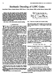
We have implemented Algorithm 1 on a random LPDC code of size n = 1000 and rate R = 3/4 and have compared the results with other existing methods. The variable node degree is dv = 3, and thus, dc = 4. The algorithm is compared with the mixed integer method of Draper and Yedidia [27], and the random facet guessing algorithm of [28]. The mixed integer algorithm re-runs the LP decoding by setting integer constraints on a small subset of “least certain” bits, namely the positions where the LP minimal pseudocodeword entries are closest to 0.5. We have taken the size of the constrained subset to be M = 5, which means the number of extra iterations is 32 for the mixed integer method. We also choose to run 20 more extra random iterations for facet guessing. In random facet guessing, a face (facet) of the polytope P is selected at random, among all the faces on which the LP minimal pseudocodeword does not reside. Then, LP decoder is re-run with the additional constraint that the solution is on the selected face. In contrast, Algorithm 1 has only one extra iteration. All methods are simulated in MATLAB where LP decoder is implemented via the cvx toolbox [29]. We have plotted the BER curves versus the probability of error p in Figure 2. For Algorithm 1, for each p, we have experimentally found the optimal λ1 and λ2 by choosing the values that on average result in the best performance. For most of the cases the chosen values where in the ranges −3 ≤ λ1 ≤ −0.5 and 1 ≤ λ2 ≤ 3. Observe the superior BER performance of Algorithm 1 which becomes more significant for smaller values of p. For p = 0.11, the BER improvement in the reweighted LP method is at least one order of magnitude. In our preliminary experimental evaluation we observe that the BER curves eventually collapse into the same curve as the LP curve, except for the reweighted LP algorithm, which is an indication of the fact that the empirical thresholds of
18
0
10
LP Random Facet Guessing Mixed Integer Draper et al. −1
Iterative Weighted LP
10
−2
BER
10
−3
10
−4
10
−5
10
0.11
0.12
0.13
0.14
0.15
0.16
0.17
0.18
0.19
0.2
p
Figure 2: BER curves as a function of channel flip probability p, for LP decoding and different iterative schemes; random facet guessing of [28], mixed integer method of [27], and the suggested iterative reweighted LP of Algorithm 1. The code is a random LDPC(3,4) of length n = 1000. Algorithm 1 are better than those of LP decoder and existing polynomial time post processing methods.
References [1] J. Feldman, “Decoding Error-Correcting Codes via Linear Programming”, PhD thesis, MIT, 2003. [2] J. Feldman, M. J. Wainwright, and D. R. Karger,“Using linear programming to decode binary linear codes,” IEEE Transactions on Information Theory, 51(3):954-972, 2005. [3] J. Feldman, D. R. Karger and M. J. Wainwright, “Linear Programming-Based Decoding of Turbo-Like Codes and its Relation to Iterative Approaches,”Proc. 40th Annual Allerton Conf. on Communication, Control, and Computing Oct. 2002. [4] M. J. Wainwright, T. S. Jaakkola and A. S. Willsky,“MAP estimation via agreement on (hyper)trees: Message-passing and linear programming approaches,” Proc. Allerton Conference on Communication, Control and Computing Oct. 2002. [5] R. Koetter and P. O. Vontobel, “Graph-covers and iterative decoding of finite length codes,” Proc. 3rd International Symp. on Turbo Codes, Sep. 2003. [6] P. O. Vontobel and R. Koetter,“Towards low-complexity linear-programming decoding,” Proc. Int. Conf. on Turbo Codes and Related Topics,Munich, Germany, Apr. 2006. [7] M. H. Taghavi and P. H. Siegel,“Adaptive linear programming decoding,” IEEE Int. Symposium on Information Theory, Seattle, WA, July 2006.
19
[8] M. P. C. Fossorier, “Iterative reliability-based decoding of low-density parity check codes,” IEEE Transactions on Information Theory, May 2001, pp:908-917. [9] H. Pishro-Nik and F. Fekri, “On Decoding of LDPC Codes over the Erasure Channel,” IEEE Trans. Inform. Theory, Vol. 50, pp:439-454 2004. [10] K. Yang, J. Feldman and X. Wang “Nonlinear programming approaches to decoding low-density parity-check codes,” IEEE J. Sel. Areas in Communication, Vol. 24 NO. 8, pp: 1603-1613, Aug. 2006. [11] M. Chertkov and V. Y. Chernyak,“Loop calculus helps to improve belief propagation and linear programming decoding of LDPC codes”, Allerton Conference on Communications, Control and Computing,Monticello, IL, Sep. 2006. [12] M. J. Wainwright and T. S. Jaakkola and A. S. Willsky,“Exact MAP estimates via agreement on (hyper)trees: Linear programming and message-passing,” IEEE Trans. Information Theory, Vol. 51, NO. 11 pp: 3697-3717, Nov. 2005. [13] J. Feldman, T. Malkin, R. A. Servedio, C. Stein, and M. J. Wainwright, “ LP decoding corrects a constant fraction of errors”, In Proc. IEEE International Symposium on Information Theory, 2004. [14] C. Daskalakis, A. G. Dimakis, R. M. Karp and M. J. Wainwright, “Probabilistic Analysis of Linear Programming decoding”, IEEE Transactions on Information Theory, Volume 54, Issue 8, Aug. 2008. [15] S. Arora, D. Steuer, and C. Daskalakis, “Message-Passing Algorithms and Improved LP Decoding”, ACM STOC 2009. [16] A.G. Dimakis and P. O. Vontobel, “LP Decoding meets LP Decoding: A Connection between Channel Coding and Compressed Sensing”, Allerton 2009. [17] A. G. Dimakis, R. Smarandache and P. O. Vontobel “LDPC Codes for Compressed Sensing”, arxiv 1012.0602. [18] D. Donoho, “High-dimensional centrally symmetric polytopes with neighborliness proportional to dimension,” Discrete and Computational Geometry, 102(27), pp. 617-652 2006, Springer. [19] D. Donoho and J. Tanner, “Neighborlyness of randomly-projected simplices in high dimensions,” Proc. National Academy of Sciences, 102(27), pp. 9452-9457, 2005. [20] A. Khajehnejad, W. Xu, S. Avestimehr, B. Hassibi, “Improved Sparse Recovery Thresholds with Two-Step Reweighted `1 Minimization”, ISIT 2010. [21] E. J. Cand´es, M. B. Wakin, and S. Boyd, “Enhancing Sparsity by Reweighted l1 Minimization”, Journal of Fourier Analysis and Applications, 14(5), pp. 877-905, special issue on sparsity, December 2008. [22] E. J. Cand`es and T. Tao, “Decoding by linear programming”, IEEE Trans. Inform. Theory, 51 4203-4215
20
[23] D.L. Donoho and X. Huo,“ Uncertainty principles and ideal atomic decomposition”, IEEE Transactions on Information Theory, 47(7):28452862, 2001. [24] M.Stojnic, W. Xu, and B. Hassibi, “Compressed sensing - probabilistic analysis of a null-space characterization”IEEE International Conference on Acoustic, Speech and Signal Processing, ICASSP 2008 [25] A. Cohen, W. Dahmen, and R. DeVore,“ Compressed sensing and best k-term approximation”, Journal of the American Mathematical Society ,Volume 22, Number 1, January 2009, Pages 211231 [26] W. Xu and B. Hassibi, “On Sharp Performance Bounds for Robust Sparse Signal Recoveries”, accepted to the International Symposium on Information Theory 2009. [27] S.C. Draper, J.S. Yedidia, Y. Wang, “ML Decoding via Mixed-Integer Adaptive Linear Programming”, IEEE International Symposium on Information Theory (ISIT), June 2007 (ISIT 2007, TR2007022). [28] A. G. Dimakis, A. A. Gohari and M. Wainwright, “Guessing Facets: Polytope Structure and Improved LP Decoder”, IEEE Transactions on Information Theory, Volume 55, Issue 8, Aug. 2009, [29] cvx toolbox webpage http://cvxr.com/cvx/.
A
Proof of Lemma 5.1
We first prove the following lemma. Lemma A.1. Suppose {τij | 1 ≤ i ≤ n, 1 ≤ j ≤ m} is a set of feasible dual variables on the edges of the factor graph G of the code C, for some arbitrary log-likelihood vector γ. Then for every vector w ∈ K(C) and every check node cj , the following holds X
wi τij ≥ 0.
(35)
vi ∈N (cj )
Proof. We only use condition (i) of a feasible set of dual variables. Note that among the variable nodes in N (cj ), there can be at most one node vi with τi,j < 0. Let vi be such a variable node. From the definition of K we can write wi ≤
X
wi0 ,
i0 ∈N (j)\i
or equivalently: τij wi +
X vi0 ∈N (vj )\i
21
|τij |wi0 ≥ 0.
(36)
Moreover, we know that τij + τi0 j ≥ 0 for i0 6= i, from the condition (i) of the dual feasibility. Therefore, replacing τi0 j with |τij | for each i0 6= i does not decrease the left hand side of (36), and thus X
wi τij ≥ 0.
vi ∈N (cj )
We now invoke Lemma A.1 that for every check node cj ,
P
vi ∈N (cj ) wi τij
≥ 0. If we sum
these inequalities for all check nodes cj we obtain: X
X
wi τij =
X vi ∈Xv
cj ∈Xc vi ∈N (cj )
X
wi
τij ≥ 0,
cj ∈N (vi )
When Xv and Xc are the sets of variable and check nodes respectively. Since τij s are feasible P dual variables, from condition (ii) of feasibility (Definition 3), we must have cj ∈N (vi ) τij < γi . It then follows that X
γi wi > 0.
vi ∈Xv
B
Proof of Theorem 5.1
We basically repeat the argument of [13] with some slight adjustments. Let S be the set of flipped bits, or interchangeably the set of corresponding variable nodes in the factor graph G (we use vi to refer to the variable node corresponding to the ith bit). Definition 9 ((δ, λ) matching from [13]). A (δ, λ) matching of the set S is a set M of edges of the factor graph G, so that no two edges are connected to the same check node, every node in S is connected to at least δdv edges of M , and every node in S 0 is connected to at least λdv edges of M . Here S 0 is the set of variable nodes that are connected to at least (1 − λ) check nodes in N (S). If there is a (δ, λ) matching on the set S, then we consider the following labeling of the edges of G. For a check node vj , if it is adjacent to an edge τij is M then set τij = −x and τi0 j = x for every other variable node vi0 ∈ N (vj ) i0 6= i. Otherwise, label all of the edges of the edges adjacent to j by 0. It can be seen that this for this labeling {τij } satisfies condition (i) of dual feasibility (Definition 3), and furthermore:
X j∈N (i)
(1 − 2δ)d x i ∈ S v τij ≤ . (1 − λ)dv x i ∈ S c 22
(37)
We know take λ = 2 − 2δ + 1/dv . Let us define a new likelihood vector γ 0 by −C i ∈ S γ0 = . 1 i ∈ Sc
(38)
If a dual feasible set exists that satisfies the feasibility condition for the vector γ 0 , then this implies that the FCP(S, C) holds. Now, since C
t, ωi appears in at most dv − q inequalities and on the right hand side. This comes directly from the definition of a (p, q)-matching on the set S. Therefore p
X i∈S
ωi ≤ (dv − p)
X
ωi + (dv − q)
X
ωi ,
(41)
i∈S c
i∈S
and thus, X 2p − dv X ωi ≤ ωi , dv − q c i∈S
i∈S
which proves that C has the desired fundamental cone property.
23
(42)
D
Proof of Theorem 5.2
We denote the set of variable nodes and check nodes by Xv and Xc respectively. For a fixed w ∈ [0, 1]T , let B be the set of all minimal T -local deviations, and Bi be the set of minimal T -local deviations that result from a skinny tree rooted at the variable node vi . Also, assume S is the random set of flipped bits, when the flip probability is p. Interchangeably, we also use S to refer to the set of variable nodes corresponding to the flipped bits indices. We are interested (S)
in the probability that for all β (w) ∈ B, fC (β (w) ) ≥ 0. Recall that (S)
fC (x) :=
X
xi − C
i∈S c
X
xi .
i∈S
(S)
For simplicity we denote this event by fC (B) ≥ 0. Since the bits are flipped independently and with the same probability, we have the following union bound � � � � (S) (S) P fC (B) ≥ 0 ≥ 1 − nP fC (B1 ) ≥ 0 .
(43)
Now consider the full tree of height 2T, that is rooted at the node v1 , and contains every node u in G that is no more than 2T distant from v, i.e. d(v1 , u) ≤ 2T . We denote this tree by B(v1 , 2T ). To every variable node u of B(v1 , 2T ), we assign a label, I(u), which is equal to −Cωh(u) if u ∈ S, and is ωh(u) if u ∈ S c , where (ω0 , ω2 , · · · , ω2T −2 ) = w. We can now see that (S)
the event fC (B1 ) ≥ 0 is equivalent to the event that for all skinny subtrees T of B(v1 , 2T ) of height 2T , the sum of the labels on the variable nodes of T is positive. In other words, if Γ1 is (S)
the set of all skinny trees of height 2T that are rooted at v1 , then fC (B1 ) ≥ 0 is equivalent to: min
T ∈Γ1
X
I(v) ≥ 0.
(44)
v∈T ∩Xv
We assign to each node u (either check or variable node) of B(v1 , 2T ) a random variable Zu , P which is equal to the contribution to the quantity minT ∈Γ1 v∈T ∩Xv I(v) by the offspring of the node u in the tree B(v1 , 2T ), and the node u itself. The value of Zu for can be determined recursively from all of its children. Furthermore, the distribution of Zu only depends on the height of u in B(v1 , 2T ). Therefore, to find the distribution of Zu , we use X0 , X1 , · · · , XT −1 as random variables with the same distribution as Zu when u is a variable node (X0 is assigned to the lowest level variable node) and likewise Y1 , Y2 , · · · , YT −1 for the check nodes. It then follows that:
24
Y0 = ω0 η, (dc −1)
(1)
Xi = min{Yi , . . . , Yi Yi = ωi η +
(1) Xi−1
+ ··· +
} ∀i > 0,
(d −1) Xi−1v
∀i > 0, (45)
where X (j) s are independent copies of a random variable X, and η is a random variable that takes the value −C with probability p and value 1 with probability 1 − p. It follows that
� � � � (S) (1) (dv ) P fC (B1 ) ≤ 0 = P XT −1 + · · · + XT −1 ≤0 ≤ (E(e−tXT −1 ))dv .
(46)
The last inequality is by Markov inequality and is true for all t > 0. The rest of the proof we bring here is basically appropriate modifications of the derivations of [15] for the Laplace transform evolution of the variables Xi s and Yi s, to account for a non-unitary robustness factor C. By upper bounding the Laplace transform of the variables recursively it is possible to show that (see Lemma 8 of [15], the argument is completely the same for our case)
Ee−tXi ≤ Ee−tXj Y
�(dv −1)i−j (dc − 1)Ee−tωi−k η
�(dv −1)k
,
(47)
0≤k≤i−j−1
for all 1 ≤ j ≤ i < T . If we take the weight vector as ω = (1, 2, · · · , 2j , ρ, ρ, · · · , ρ) for some integer 1 ≤ j < T , and use equation (47), we obtain:
T −j−1
Ee−tXT −1 ≤ (Ee−tXj )(dv −1)
· (dc − 1)Ee−tρη
� (dv−1)T −j−1 −1 dv −2
.
ρ and t can be chosen to jointly minimize Ee−tXj and Ee−tρη in the above, which along with
25
(46) results in P(fCS (B1 ≤ 0)) ≤ (Ee−tXT −1 )dv ≤ γ −dv /(dv −2) × cdv (dv −1)
T −j−1
,
C.p 1/(C+1) where γ = (dc − 1) C+1 and c = γ 1/(dv −2) mint≥0 Ee−tXj . If c < 1, then C (1 − p)( 1−p )
probability of error tends to zero as stated in Theorem 5.2.
26