Network Center Selection. Dae-Won Lee and Jaewook Lee. Department of Industrial Engineering,. Pohang University of Scien
A Novel Three-Phase Algorithm for RBF Neural Network Center Selection Dae-Won Lee and Jaewook Lee Department of Industrial Engineering, Pohang University of Science and Technology, Pohang, Kyungbuk 790-784, Korea. {woosuhan,jaewookl}@postech.ac.kr
Abstract. In this paper, we propose a new method for selecting RBF centers. The strength of our method is to determine the number and the locations of RBF centers automatically without any priori assumption about the number of centers. The proposed method consists of three phases. The first phase is to partition the input patterns into the several subsets according to their output labels. In the second and third phase, the number and the locations of RBF centers are determined using bisection algorithm and weighted mean centering. These second and third phase are iteratively repeated until to reach the goal error. The proposed method is applied to several benchmark data sets. The numerical results show that our method is robust and efficient for determining the number and the locations of centers.
1
Introduction
Radial basis function network (RBFN), due to the simplicity of its single hidden layer structure and universal property, has been widely used for nonlinear function approximation and pattern classification. Training of the RBFNs consists of selecting centers of the hidden neurons and estimating the weights that connect the hidden and the output layers. Once centers have been fixed, the network weights will be directly estimated by using the least squares algorithm. The generalized radial basis function network(GRBFN) involves searching for a suboptimal solution in a lower-dimensional space that approximates the interpolation solution where the approximated solution F ∗ (x) can be expressed as follows F ∗ (x) =
m �
wi φ(�x − ti �)
(1)
i=1
where the set of RBF centers {ti |i = 1, . . . , m} is to be determined. One of the key issues in the design of RBFN specially is how to determine the number and the locations of the RBF centers. In the recent researches, a variety of ways for determining the locations of centers have been proposed. Previously reported approaches for RBF center selection include random selection from F. Yin, J. Wang, and C. Guo (Eds.): ISNN 2004, LNCS 3173, pp. 350–355, 2004. c Springer-Verlag Berlin Heidelberg 2004 �
A Novel Three-Phase Algorithm
351
input patterns [1], and selection of centers based on clustering algorithms [2], [3]. These methods have some drawbacks in that they cannot determine the number and the locations of centers at the same time and do not consider the information of the supervised data. In this paper, to overcome such drawbacks, the proposed method consists of three basic ingredients. Firstly, input patterns are partitioned into several subsets according to their output labels and the RBF centers are determined separately for each subset in order to reflect information of the output class label. Then these centers are combined to form a larger superset to be used in the final RBFN. Secondly, the proposed algorithm determines the number of the centers by using bi-section algorithm. Finally, the proposed algorithm determines the optimal locations of the centers by employing a weighted mean centering. The organization of this paper is as follows : In Section 2 a new method for RBF center selection was explained. Section 3 presents an algorithm for the proposed method, and Section 4 presents experimental results applied to benchmark problems, followed by conclusions in Section 5.
2 2.1
The Proposed Method Phase I: Partitioning Supervised Data
The proposed method is basically similar to the selection of centers based on clustering algorithm which is most widely used for center selection. However this kind of approaches deal with input patterns as unsupervised data during the center selection step even though supervised data are available. When the output class label is not considered, some of centers is often found to be located in the boundary between several classes, in which case these centers fail to play a role of a good feature extractor in the GRBFN. In phase I, we partition training data into C disjoint subsets {Di }C i=1 according to its class to reflect the distribution of input pattern for each output class. Then, with each subset, cluster centers are found using clustering algorithm to be explained in Section 2.2 and 2.3. Finally, we use C disjoint sets of cluster centers as GRBFN centers. 2.2
Phase II: Determining the Number of Centers by Bi-section Algorithm
Phase II tries to estimate the proper number of centers automatically. The idea was originated from Cover’s theorem on the separability of patterns [4]: the more GRBFN has hidden neurons, the more input patterns are linearly separable. It can be interpreted that a training error rate curve against the number of centers is approximately monotonic decreasing function. From this observation, in order to find the number of centers we employed the bi-section algorithm expressed in Fig.1. It can approximately estimate the minimum number of centers reaching the goal error rate with reducing the search space (1 ∼ N ) in a ratio of 1/2. One advantage of this algorithm is that it can find the number of centers within a comparatively less time because it has only O(log2 N ) complexity.
352
D.-W. Lee and J. Lee
Fig. 1. Flow diagram for center selection (Phase II and III). Where Error(λ) is a misclassified rate with the λ number of centers
2.3
Phase III: Determining the Locations of Centers Using Weighted Mean Centering
Determining the locations of the RBF centers is based on optimizing the following objective function with respect to (t, w). E=
N 1�
2
di −
i=1
ki �
2 wj φ(�xi − tj �)
(2)
j=1
From the necessary optimality condition, positions of centers is given by N
� ∂E 1 = 2 wj (d − Φw)i Φij (xi − tj ) = 0 ∂tj σ i=1 �N tj = =
i=1 (d − Φw)i Φij xi �N i= (d − Φw)i Φij
N �
λj (xi , t, w)xi ,
=
N � i=1
�
(d − Φw)i Φij
�N
i=1 (d
− Φw)i Φij
(3) � xi (4)
∀j = 1, . . . , ki
i=1
�N where i=1 λj (xi , t, w) = 1, ∀j = 1, . . . , ki , Φ = [φ(xi , tj )]i=1,... ,ni , j=1,... ,ki , d = [d1 , d2 , . . . , dN ]T and w = [w1 , w2 , . . . , wm1 ]T . It shows that the estimate for tj is merely a weighted average of the samples. However, due to the highly non-linearity of E with respect to the centers tj , it is very difficult to compute
A Novel Three-Phase Algorithm
353
tj directly. Instead, we employ a so-called weighted mean centering scheme to implement this, which consists of two steps. In the first step, center positions tj of Eq. (4) are approximated as a simple average of the xi that has higher absolute value of the numerator of λj (xi , t, w). This process is repeated until no change is made. (See Section 3 for more details about this.) In the case of non-convex data set, the obtained centers in the first step are often found to be located in the regions of other classes, even though we have partitioned data sets according to their classes. To avoid this problem, in the second step, we modify RBF centers into the nearest points within the partitioned subset Di .
3
Algorithm
An algorithm of center selection for the proposed method is as follows. % Phase I: Partitioning supervised data 1. Separate N training data into C disjoint subsets Di containing ni elements, according to class. {(xi , di )}N i=1 → D1 ∪ D2 ∪, . . . , ∪DC Di = {(x1 , i), (x2 , i), . . . , (xni , i)} for i = 1, . . . , C % Selecting ki centers for each subset Di 2. for i = 1 to C do % Phase II: bi-section algorithm 2.1. Determine the number of centers (ki ) using bi-section algorithm as i explained in Fig. 1: initially, ki = 1+n 2 . % Phase III: weighted mean centering 2.2. Determine the locations of ki centers using weighted means centering. ki from input 2.2.1. Choose random values for the initial centers Ti = {tj }j=1 space. Where tj is the jth cluster center of subset Di . % Adjust the centers 2.2.2. for l = 1 to ni do 2.2.2.1. Let Ii (xl ) denote the index of the best-matching center for the input vector xl ∈ Di as follows. Ii (xl ) = arg max �(d − Φw)l Φlj �, j
j = 1, 2, . . . , ki
2.2.2.2. Adjust the centers using the update rule tj ← tj + η(xl − tj ),
j = Ii (xl )
(5)
where η is a learning step size. 2.2.3. Continue the center adjusting procedure (step 2.2.2) until no change i are observed in the centers {tj }kj=1 2.2.4. Modify centers into nearest points of partitioned subset Di and determine final locations of centers.
354
D.-W. Lee and J. Lee Table 1. Benchmark data description
2-Spirals Sonar Heart Vowel
Input dimension Number of classes Number of patterns 2 2 388 [194,194] 60 2 104 [55,49] 13 2 180 [98,82] 10 11 528[48,48,48,48,48,48,48,48,48,48,48]
bracketed numbers mean the number of patterns for each class.
tj = the nearest point x ∈ Di for j = 1, 2, . . . , ki 2.3. Repeat Step 2.1.∼2.2. until converge to goal error. % Complete the RBFN training 3. Combine the centers of C disjoint subsets {Di }C i=1 and construct generalized RBF network by using pseudo-inverse. T = {tj }K j=1 ← T1 ∪ T2 ∪, . . . , ∪TC w = (ΦT Φ + λΦ0 )−1 ΦT d where Φ = [φ(xi , tj )]i=1,... ,N, �C i=1 ki .
4
j=1,... ,K ,
Φ0 = [φ(xi , tj )]i,j=1,... ,K , and K =
Simulation Results
The algorithm described in the previous section has been simulated on four kinds of benchmark data sets (2-spiral, sonar, heart, vowel). Description of the benchmark data sets is given in Table 1. The performance of the proposed method is compared with two widely used center selection methods. In Table 2, KM is the k-means based center selection without partitioning and RS is random selection from training data without partitioning. For these two methods, the number of centers is determined by increasing centers one by one until they achieve the goal error. For the comparison we adopted three criterion: the number of centers, the mis-classified rate, and the computing time. Simulation results are shown in Table 2. The results show that the proposed method achieves better accuracy with a slightly fewer number of RBFN centers while significantly reducing computing time.
5
Concluding Remarks
In this study, we have presented a novel three-phase algorithm for RBF center selection. The proposed method has several advantages. Firstly, it determines the number and the locations of centers automatically without any assumption about the number of centers. Secondly it selects good feature extractors by using
A Novel Three-Phase Algorithm
355
Table 2. Simulation results on four benchmark problems Method m 2-Spiral 84 Sonar 37 Heart 129 Vowel 66
KM E 0.069 0.096 0.97 0.099
T 5650 1570 11876 3658
m 88 37 131 64
RS E 0.080 0.096 0.99 0.099
Proposed T m 80 [35,45] 5925 1112 34 [17,17] 9723 129 [68,61] 2465 59 [2,5,5,2,8,7,3,2,9,2,14]
E 0.064 0.096 0.093 0.099
T 297 21 125 188
m is the number of centers and bracketed numbers are the number of centers for each class. E is mis-classified error rate and T is computing time to construct the GRBFN.
the information of output class label. Finally, it is robust to a data set with nonconvex distribution. Experimental results show that the proposed method is competitive with the previously reported approaches for RBF center selection. Other methods to improve efficiency of RBF center selection, such as Homotopy method [5], [6] can be also be investigated.
Acknowledgement. This work was supported by the Korea Research Foundation under grant number KRF-2003-041-D00608.
References 1. Mao, K.Z.: RBF Neural Network Center Selection Based on Fisher Ratio Class Separability Measure. IEEE Trans. Neural Networks, Vol. 13(5) (2002) 1211-1217 2. Gomm, J.B., Yu, D.L.: Selection Radial Basis Function Network Centers with Recursive Orthogonal Least Squares Training. IEEE Trans. Neural Networks, Vol. 11(2) (2000) 306-314 3. Haykin, S.: Neural Networks: A Comprehensive Doundation. Prentice Hall, New York (1999) 4. Cover, T.M.: Geometrical and Statistical Properties of Systems of Linear Inequalities with Applications in Pattern Recognition. IEEE Trans. Electronic Computers, Vol. EC-14 (1965) 326-334 5. Lee, J., Chiang, H.-D.: Constructive Homotopy Methods for Finding All or Multiple DC Operating Points of Noninear Circuits and Systems. IEEE Trans. on Circuits and Systems- Part I, Vol. 48-(1) (2001) 35-50 6. Lee, J., Chiang, H.-D.: A Singular Fixed-Point Homotopy Method to Locate the Closest Unstable Equilibrium Point for Transient Stability Region Estimate. IEEE Trans. on Circuits and Systems- Part II, Vol. 51-(4) (2004) 185-189