A NUMA-aware fine grain parallelization framework for multi-core architecture Corentin Rossignon, H´enon Pascal, Olivier Aumage, Samuel Thibault
To cite this version: Corentin Rossignon, H´enon Pascal, Olivier Aumage, Samuel Thibault. A NUMA-aware fine grain parallelization framework for multi-core architecture. PDSEC - 14th IEEE International Workshop on Parallel and Distributed Scientific and Engineering Computing - 2013, May 2013, Boston, United States. 2013.
HAL Id: hal-00858350 https://hal.inria.fr/hal-00858350 Submitted on 5 Sep 2013
HAL is a multi-disciplinary open access archive for the deposit and dissemination of scientific research documents, whether they are published or not. The documents may come from teaching and research institutions in France or abroad, or from public or private research centers.
L’archive ouverte pluridisciplinaire HAL, est destin´ee au d´epˆot et `a la diffusion de documents scientifiques de niveau recherche, publi´es ou non, ´emanant des ´etablissements d’enseignement et de recherche fran¸cais ou ´etrangers, des laboratoires publics ou priv´es.
A NUMA-aware fine grain parallelization framework for multi-core architecture Corentin Rossignon Total - E&P CSTJF Pau, France
[email protected]
Pascal H´enon Total - E&P CSTJF Pau, France
[email protected]
Abstract—In this paper, we present some solutions to handle two problems commonly encountered when dealing with fine grain parallelization on multi-core architecture: expressing algorithm using a task grain size suitable for the hardware and minimizing the time penalty due to Non Uniform Memory Accesses. To evaluate the benefit of our work we present some experiments on the fine grain parallelization of an iterative solver for sparse linear system with some comparisons with the Intel TBB approach. Keywords-task flow; scheduler; aggregation; fine-grain parallelism; NUMA
Olivier Aumage Inria Runtime project team Bordeaux, France
[email protected]
runtime scheduler is then in charge of launching tasks on the hardware and achieve a good load-balancing. Nevertheless, these programming models lack some features to handle efficiently some important classes of problems. Indeed, very often two crucial problems have to be addressed in order to achieve an efficient fine grain parallelization: •
I. I NTRODUCTION With the commoditization of multi-core processors in clusters, the inter-node parallelism expressed by HPC applications needs to be complemented by a finer-grained parallelism that takes advantage of shared memory at the intra-node level. The fine grain parallelism means that we can exhibit new levels of parallelism by parallelizing some operations that are usually done sequentially. Usually it consists to parallelize some algorithms done inside a MPI process by using several cores of a cluster node. Indeed by taking advantage of the shared memory at the node level, some algorithms are then parallelizable whereas they could not be efficiently parallelized using the static partitioning of data and communication overhead imposed by a distributed memory framework (e.g., MPI). Some popular shared memory parallel frameworks like Intel TBB [1], Cilk [2] or OpenMP 3.0 [3] propose programming models that considerably alleviate the fine grain parallelization in a shared memory environment. Those models rely on the use of a scheduler that dispatches the computation tasks at runtime on the available cores of a cluster node. The simplest form of fine grain parallelism consists in splitting independent works done in a loop among the cores. More complex algorithms require to expose the parallelism as an Direct Acyclic Graph (DAG) where each node is a task consists in a group of operations that can only be computed when all its predecessor tasks has been completed. With such a computational task graph approach, the work that falls to the developer is to describe the computations as a collection of tasks and to give the set of predecessor and successor tasks for each of them. The
Samuel Thibault Universit´e Bordeaux I Runtime project team Bordeaux, France
[email protected]
•
The first one is to obtain a correct task grain size for a good parallel efficiency: a too fine parallelism grain leads to bad performances caused by the task management and scheduling overhead while a too coarse grain does not provide enough parallelism for the hardware capability and causes load balancing issues. The second problem is to take into account the Non Uniform Memory Accesses (NUMA) that are caused by the time penalty when a core needs to access some data that are not physically located on a memory bank directly linked to its socket. Therefore the physical location of memory allocation needs to be carefully driven to match the task scheduler policy in order to minimize these time penalties.
In this paper, we present some solutions to handle these two problems at the level of the programming model. Our main motivation is that we want a programming model that adds as few as possible efforts starting from a natural task based parallelization of an algorithm (using TBB for example) to obtain a better efficiency by taking care of NUMA and task grain size. To evaluate the benefit of our work we present some experiments on the parallelization of an iterative solver for sparse linear systems. A popular approach to solve large sparse linear systems of equations is a Krylov method (like GMRES or Conjugate Gradient) preconditioned by an incomplete factorization (see [4]). This is often the most time consuming part of a numerical simulation. The usual way to parallelize this kind of solvers is to use a weaker form of the preconditioner in parallel by preconditioning subdiagonal blocks of the matrix: the subdiagonal block are usually obtained thank to a partition of the adjacency graph of the matrix. Outside the preconditioner, the operations required in a Krylov method are vector operations (mostly
BLAS1 type like dot products or AXPY) and matrix vector products: those operations are naturally dealt with parallel loop splitting (e.g., parallel for in OpenMP). In this paper, we have chosen to focus on the fine grain parallelization of the ILU preconditioner. In this case, more levels of parallelism can be obtained because the factorization and triangular solves of a submatrix can be parallelized on several cores. Incomplete factorization and associated triangular solve of a sparse matrix is a problem that is well representative of the difficulty that one can encounter with fine-grain parallelization: the fine grain description of these algorithms is natural but in practice a straight task based parallelization using TBB or OpenMP does not give good speed-up because of the very low computational cost of a task and the NUMA effect when accessing the coefficients of the matrix and vector. In the experiment results, we will evaluate our programming model on those algorithms. The paper is organized as follows. Section II expresses the problem statement of task grain tuning, NUMA effect and then discusses existing and past works related to these problems. Section III explains how we propose to improve existing task based programming models to deal with these problems. Section IV shows the benefit of our work on the fine-grain parallelization of an ILU(k) factorization and the triangular solves associated with the sparse LU decomposition of the matrix. Sections V and VI present experimental results on a NUMA platform compared to TBB (OpenMP has very similar performance on those problems). Section VII concludes the paper, and presents ongoing and intended future works. II. P ROBLEM S TATEMENT The principle of using tasks to express the potential application parallelism in an abstract way, independent from available hardware resources, was once popularized by tools such as Cilk [2]. The widespread availability of multi-core processors recently revived the popularity of task scheduling frameworks [5] as exemplified by tools such as Intel TBB [1] and OpenMP 3.0’s task support [6] for regular multicore platforms, or StarSs/OmpSs derivatives [7] as well as StarPU [8] and X-Kaapi [9] for heterogeneous platforms. Most frameworks for multi-core platforms don’t handle memory locality, some try to improve data locality between tasks by letting the user the choice of the next task to schedule (e.g., continuation in TBB). In case of tasks scheduler for heterogeneous platforms, data need to be moved to the target platform. Therefore, in this case, the scheduler must know which data are used by each task to move them at the right moment, unfortunately none of these schedulers care about NUMA in their scheduling algorithms to reduce the overhead of data displacement. Several related works have been conducted in the past to address the issue of adapting the task grain size to the amount of available computing units. Many related works
partially address this grain size issue by promoting cacheoblivious techniques for a specific class of applications such as recursive, divide-and-conquer codes or recursively partitioned loops [1], [2], [5], [9], [10]. Works such as the SCOOPP framework [11] provides means for the applications to control the task grain size. However, the grain size selection issue is still up to the application programmer. On the theoretical side, general task scheduling has been heavily studied for a long time now [12], [13]. Works on task grain adaptiveness have been scarcer but do exist. The work presented in this paper is built on grain-packing [14] and task clustering [15] past works. III. TASK - GRAIN TUNING THROUGH G UIDED AGGREGATION To solve the granularity problem, several possible approaches exist. We could enable task parallelism only when cores are idle. For example, X-Kaapi [9] uses this approach with its adaptive task model, this is a very good solution with parallel loops or tree task flow. But in general case, the user needs to define a function that splits the task flow graph into two complete parallel parts, which is not always possible. Another possible approach, as given by Capsules [16], requires the user to define several grain sizes. The runtime then chooses which grain best matches the current situation. The application programmer must therefore design his/her application while having these multiple granularity levels in mind, which may prove difficult to realize or express in an abstract way in the code. Our approach is different. From the finest-grained DAG, we build a coarse-grained DAG after the machine topology layout and the run-time state using an aggregate operator on subsets of tasks. Our default aggregate operator just serializes the function called within all merged tasks. But the aggregate operator itself is user programmable by overloading the aggregate method of our task class. Indeed it is often interesting to redefine this operator: for example instead of calling sequentially several functions that depend on a parameter i it is more efficient to use a single function call that loops on the list of i parameters. Several possible aggregate operators are experimented later in this paper. Those aggregate operators are called from a dedicated framework called Taggre which interfaces with existing low-level task schedulers. Taggre expects a fine grain task DAG as input. It then returns a coarser DAG as the result of applying the selection of aggregate operators on the contents of the fine-grain DAG. A. Aggregate operator algorithms As a proof of concept, we have defined several heuristics that coarses the DAG to change the task grain size. Multiple heuristics may be chained together to further coarsen the
0
0 0 1
1
2
3
0-3
1-2 2
3-4
4
3
8 4-7
4 5
6
9
8-11
10
5 5
7
Figure 1: Example of aggregation with S algorithm 0
1
2
11
Figure 3: Example of aggregation with D algorithm and parameter 4
0
3
4
1-2
3-4
Figure 2: Example of aggregation with the F algorithm and parameter 2
DAG. In Taggre, each algorithm is thus designated by a letter. The sequence of selected letters is called the Coarse String. For example, the Coarse String “SD(300)F(32)” means the call of Sequential algorithm, followed by the Depth Front algorithm with parameter 300 and finally by the Front algorithm with parameter 32. The parameters are algorithm-dependent. 1) Sequential (S): This is the most straightforward algorithm. We aggregate tasks having a single predecessor with their predecessor, if such a predecessor has a single successor (Fig. 1). 2) Front (F): This algorithm takes one argument which is the maximum number of tasks per depth level. We call this number N . The basic idea of this algorithm is to limit the number of simultaneously available tasks and thus to limit the oversubscription of computing units. To do this, the Front algorithm implements a breadth-first traversal of the DAG. During the traversal, it aggregates tasks of same depth to group the maximum of N coarse tasks of similar computation time (e.g., grain size) per depth (Fig. 2). 3) Depth Front (D): This algorithm expects one argument which is the maximum number of fine grain tasks aggregated into a coarse grain task. We call this number M . The main idea of this algorithm is to aggregate a task with some of its descendants, up to the limit M . For that, the algorithm performs a breadth-first traversal of the descendants of a task to aggregate up to M tasks together. However, during the traversal, each new level encountered is sorted, from the task having the highest number of predecessors in the current aggregate being built, to the task having the least predecessors in this aggregate. The rationale of this heuristics is to favor aggregating tasks that are more tightly
connected in the DAG (Fig. 3). The first loop of Algorithm 1 is a loop for each level of the coarsened DAG. The second loop is a loop over tasks of the same level in coarsened DAG. Other tasks will be aggregated to these tasks in the third loop, we call them Master and they will be kept in the final DAG. The third loop is the aggregation loop, we aggregate tasks descendants of the Master task to it. Algorithm 1 Depth Front Require: M , DAG Ready = empty list put root tasks of DAG in Ready while Ready not empty do Depth = Ready Ready = empty list while Depth is not empty do Master = pop first from Depth Release = empty list put Master in Release count: 0 while count < M AND Release is not empty do Next = pop first from Release count++ aggregate Master and Next put tasks released by Next in Release, sorted by number of precedence of Master end while put tasks released by Master in Depth end while put tasks released by Depth in Ready end while 4) Continuation Oriented (C): The Continuation Oriented algorithm is an aggregation method which improves serial accesses to data inside an aggregated task. For a 3D cube, it’s equivalent to putting tasks with the same (x,y)
coordinates together. IV. A PPLICATION TO A SPARSE LINEAR SOLVER To illustrate the benefit of aggregation, we propose to study the parallelization of an iterative solver for sparse linear system. A popular approach to solve large sparse linear systems of equation is a Krylov method (like GMRES or Conjugate Gradient) preconditioned by an incomplete factorization (see [4]). This is often the most time consuming part of a numerical simulation. In this method there is two major operations, the first step is the ILU matrix factorization and the second step is the triangular solve. Outside the preconditioner, the operations required in a Krylov method are mostly BLAS1 operations and matrix vector products which naturally dealt with parallel loop splitting. In our experiments, we focus on the fine grain parallelization of the ILU preconditioner; that is to say the factorization of the matrix (done once per system solve) and the triangular system solves (done once at each iteration of the system solve). Both of those algorithms (factorization and triangular solve) can naturally be represented as a task graph. For example in the factorization a task corresponds to the factorization of a matrix row and the dependencies are directly given by the non-zero pattern of the matrix. Indeed, to factorize the row i, we need to factorize all the rows j lower than i such that the entry (i, j) is non-zero. Therefore the DAG description is easily built from the non-zero pattern of the matrix: the task i corresponds to row i of the matrix, the predecessor tasks of task i are given by the column index of non-zero coefficients before the diagonal in row i and successor tasks of task i are given by the row index of nonzero coefficients below the diagonal in the column i. Incomplete factorization and associated triangular solve of a sparse matrix is a problem that is well representative of the difficulty that one can encounter with fine-grain parallelization: the fine grain description of these algorithms is natural but in practice a straight task based parallelization using TBB or OpenMP does not give good speed-up because of the very low computational cost of a task and the NUMA effect when accessing the coefficient of the matrix and vector. In the experiment results, we will evaluate our programming model on those algorithms. Our testing machine is composed of two Intel Xeon X5570 (Nehalem) 4-core sockets with 24 GB RAM (12 GB per socket) running Red Hat Enterprise Linux 5.2 with a Linux kernel 2.6.18. The compiler used is Intel C++ compiler XE 13 with level 3 optimizations. The back-end task scheduling runtime is TBB. We obtain comparable results using OpenMP tasks. We perform the tests on two linear systems. The first one, Cube 100, is a system obtained from a 7 points discretization scheme (e.g., finite volume) of regular 3D cubes with 100 points along each dimension. It is a scalar system;
each row of the matrix is a vector of coefficients stored in double precision. The second one, SPE10, corresponds to a 7 points discretization of a reference problem from petroleum industry [17]. In this case each entry of the matrix is a small dense block (3, 3) of coefficients stored in double precision. Due to the geometry of the problem, for Cube 100, the task dependency graph is very regular whereas it is an irregular one in the SPE10 case. The characteristics of the matrices are listed in Table I. Table I: Matrices used in tests. Name
Cube 100
SPE10
Rows (n)
1,000,000
3,283,263
Number of non-zeros (nnz)
6,940,000
67,303,269
Entries of the matrix
Scalars
(3, 3) dense blocks
Each fine grain task performs one elementary line operation. SPE10 tasks weight 2-5 times more than Cube 100 tasks. However, both cases generate approximately 1 million tasks each. The test protocol is the following: • Each test is run three times, the final retained result is computed as the average of the three measured results. For each test, we collect three different timings: factorization time, triangular solve time, and aggregation time. • We perform the tests on a single socket (using numactl –cpunodebind) and on two sockets. • We test two orderings (set of row/column permutations): a natural ordering which corresponds to no modification on matrix structure where unknowns are sequentially ordered by plane following the geometric z axis (this leads to a perfect seven diagonals pattern for Cube 100) and a nested dissection [4] ordering which exposes more parallelism. • We test three levels of ILU(k) fill: 0, 1 and 2. The level k of ILU(k) preconditioner determines the level of fill of the matrix, in others words, computation per line and the number of dependencies between tasks grow up with a greater k. Table II gives the number of edges resulting in the DAG of the factorization (triangular solve DAG has a similar number of edges) for ILU(0), ILU(1) and ILU(2). Subsection IV-A will also give some features on the cost of a computational task (one row factorization) depending on the ILU level of fill parameter. • For the parameterized aggregation heuristics, we select the parameter values leading to the best performance result. With natural ordering, we can use the Cache Oriented algorithm because of particular DAG structure. With nested dissection ordering, the Cache Oriented algorithm can’t be used, so we use the Depth Front algorithm with a high value.
Table IV: Results on the ILU(k) factorization step on a single 4-core socket with TBB with nested dissection ordering.
In all tables, best results are represented in bold. Table II: Number of edges in computation DAG
Matrix
ILU
Sequential (second)
No agg.
F(32) D(400) (speed-up)
Matrix
ILU
Edges
CUBE 100 Natural ordering
ILU(0) ILU(1) ILU(2)
2,970,000 5,910,300 10,761,498
CUBE 100
ILU(0) ILU(1) ILU(2)
0.129 0.495 0.828
0.46 1.29 1.74
2.17 1.70 1.94
2.26 2.78 3.12
SPE10 Natural ordering
ILU(0) ILU(1) ILU(2)
2,970,000 5,910,300 11,357,865
SPE10
ILU(0) ILU(1) ILU(2)
0.276 1.375 2.247
0.74 1.98 2.43
1.93 1.67 1.85
2.16 2.82 3.12
A. ILU(k) Factorization Step The first test series is performed on the ILU(k) factorization step on a single 4-core socket (Tables III, IV). With aggregation disabled the task-parallel ILU(0) factorization is always slower than the sequential version, this is due to the additional cost of task management. Tasks duration for CUBE 100 in ILU(0) is only 50 ns and 240 ns for SPE10, but one task management duration is approximately 500 ns. In ILU(2), tasks are bigger, their duration is 600 ns for CUBE 100 and 1.7 µs for SPE10 but it’s not enough bigger to consider task management negligible. Another important aspect of the ILU factorization and triangular solve is that on our testbed machine the algorithm speed-up is bounded by the memory bandwidth: therefore the maximum theoretical speed-up achievable by such algorithms on several cores is less than the number of cores used. With aggregation enabled and CD(4) coarse strategy string, we now reduce the number of tasks to 2,500 with a task duration 400 times bigger. In ILU(0) we achieve a moderate speed-up of 2. ILU(2) factorization achieves a better speed-up of 3. The Front algorithm is not as effective as the Depth Front in this test case because it doesn’t aggregate tasks with continuous lines which cause many cache misses. With the Front algorithm (F(32)) in ILU(0) with natural ordering, we aggregate a maximum of 157 tasks together and, in average, we aggregate only 53 tasks. Table III: Results on the ILU(k) factorization step on a single 4-core socket with TBB with natural ordering. Matrix
ILU
Sequential (second)
No agg.
F(32) CD(4) (speed-up)
CUBE 100
ILU(0) ILU(1) ILU(2)
0.056 0.142 0.611
0.20 0.46 1.30
1.06 1.54 2.58
2.23 2.81 3.47
SPE10
ILU(0) ILU(1) ILU(2)
0.262 0.721 1.936
0.65 1.39 1.87
1.89 2.30 2.19
3.09 3.22 3.32
With two 4-core sockets (Tables V, VI), the parallel ILU(0) again performs slower than sequential execution when aggregation is disabled. With aggregation enabled, the ILU(0) achieves a speed-up of 3. ILU(2) achieves a speed-up of 6.2. Table V: Results on the ILU(k) factorization step on two 4-core sockets with TBB with natural ordering. Matrix
ILU
Sequential (second)
No agg.
F(32) CD(4) (speed-up)
CUBE 100
ILU(0) ILU(1) ILU(2)
0.056 0.143 0.612
0.28 0.65 1.47
1.27 1.89 3.06
2.54 3.79 3.91
SPE10
ILU(0) ILU(1) ILU(2)
0.260 0.771 2.006
0.97 2.24 3.37
2.48 3.80 3.97
3.78 5.72 6.21
Table VI: Results on the ILU(k) factorization step on two 4-core sockets with TBB with nested dissection ordering. Matrix
ILU
Sequential (second)
No agg.
F(32) D(400) (speed-up)
CUBE 100
ILU(0) ILU(1) ILU(2)
0.127 0.483 0.817
0.41 1.31 1.96
3.10 2.70 3.18
3.31 4.77 5.46
SPE10
ILU(0) ILU(1) ILU(2)
0.277 1.452 2.347
0.71 2.48 3.29
2.59 2.81 3.12
3.09 5.00 5.57
B. Triangular Solve Step The triangular solve step is itself composed of two parts: A forward substitution followed by a backward substitution. The DAG of the forward substitution is identical to the DAG of the factorization step mentioned in the previous section. Thus we can reuse the same coarse DAG. In our test cases, the DAG of the backward substitution part is the transpose of the DAG of the forward substitution. Here again, the factorization coarse DAG can thus straightforwardly be reused. In total we have twice more tasks in triangular solve than in factorization.
The weight of operations done in triangular solve elementary tasks is lighter than their factorization task counterparts. Tests on a single 4-core socket (Tables VII, VIII) show that the parallel triangular solve is always slower than the sequential version with task aggregation disabled. With aggregation enabled, we obtain a speedup of 2. Table VII: Results on the Triangular Solve step on a single 4-core socket with TBB with natural ordering. Matrix
ILU
Sequential (second)
No agg.
F(32) CD(4) (speed-up)
CUBE 100
ILU(0) ILU(1) ILU(2)
0.092 0.117 0.163
0.23 0.27 0.34
0.88 0.82 0.92
1.90 1.97 2.05
SPE10
ILU(0) ILU(1) ILU(2)
0.219 0.353 0.554
0.40 0.62 0.85
1.08 1.37 1.58
1.93 2.22 2.39
Table VIII: Results of the Triangular Solve step on a single 4-core socket with TBB with nested dissection ordering. Matrix
ILU
Sequential (second)
No agg.
F(32) D(400) (speed-up)
CUBE 100
ILU(0) ILU(1) ILU(2)
0.107 0.150 0.171
0.20 0.31 0.34
1.19 0.94 0.95
1.34 1.39 1.50
SPE10
ILU(0) ILU(1) ILU(2)
0.249 0.430 0.500
0.37 0.65 0.72
1.39 1.32 1.35
1.52 1.77 1.89
On two 4-core sockets (Tables IX, X), with task aggregation disabled, only the SPE10 test achieves a speedup greater than 1. With aggregation enabled, a speedup of 2.52 is achieved on ILU(0) and a speedup of 4.14 is achieved on ILU(2). Table IX: Results of the Triangular Solve step on two 4-core sockets with TBB with natural ordering. Matrix
ILU
Sequential (second)
No agg.
F(32) CD(4) (speed-up)
CUBE 100
ILU(0) ILU(1) ILU(2)
0.092 0.123 0.174
0.27 0.35 0.45
1.27 1.54 1.40
2.44 2.82 2.98
SPE10
ILU(0) ILU(1) ILU(2)
0.219 0.408 0.658
0.53 0.96 1.38
1.63 2.39 2.79
2.52 3.77 4.14
C. Aggregation Overhead This section evaluates the overhead caused by the task aggregation step for several aggregation algorithm instances. As mentioned in the test description above, the fine-grain
Table X: Results of the Triangular Solve step on two 4-core sockets with TBB with nested dissection ordering. Matrix
ILU
Sequential (second)
No agg.
F(32) D(400) (speed-up)
CUBE 100
ILU(0) ILU(1) ILU(2)
0.107 0.156 0.180
0.18 0.32 0.36
1.41 1.36 1.37
1.67 1.92 2.08
SPE10
ILU(0) ILU(1) ILU(2)
0.249 0.496 0.578
0.35 0.80 0.90
1.64 2.12 2.19
1.82 2.71 2.90
DAG generated from the test cases amount to about 1 million nodes for each matrix. The number of edges increases when the parameter k of ILU(k) preconditioner increases (see Table II). This aggregation step is performed only once for each matrix. Then, the coarsened DAG is reused as long as the sparse pattern of the matrix is unchanged. In classical numerical simulation the mesh on which the equations are discretized does not change through the simulation, only the coefficients of the linear system are changing: this means that typically the aggregation step is done only once where the factorization and triangular solves are called a large number of times (several thousand of times). The time spent in the task aggregation (Table XI) is then usually negligible compared to the time spent in the factorizations and triangular solves. In average, applying CD(4) Coarse String takes 1.5 s on a DAG with 1 million of nodes and applying D(400) takes 3.5 s. For CD(4) aggregation we won in average 0.22 s per factorization and 0.31 s per triangular solve compared to not doing aggregation. So after only 3 combinations of factorization and triangular solve, the aggregation become profitable. For D(400) aggregation we won in average 0.28 s per factorization and 0.49 s per triangular solve. So after only 5 combinations of factorization and triangular solve, the aggregation becomes profitable. V. NUMA In this section, we further improve on the previous results by taking into account the NUMA (Non Uniform Memory Access) characteristics of the testbed machine: both 4-core sockets have a faster access to their own memory bank than to the opposite socket’s memory bank (Fig. 4). In a general way, a program allocates memory from a virtual address space split into pages. Each page used by the program is transparently mapped to a physical memory location. Thus, some virtual pages can also be moved from one physical location to another one, while the virtual/physical mapping is transparently updated accordingly to the operating system without affecting the execution of
Table XI: Aggregation overhead. Matrix
ILU
F(32)
D(400) (second)
CD(4)
CUBE 100 No ordering
ILU(0) ILU(1) ILU(2)
1.534 1.467 1.871
2.945 3.032 3.705
0.908 1.119 1.315
CUBE 100 Nested dissection
ILU(0) ILU(1) ILU(2)
1.208 2.194 3.182
2.330 3.224 3.554
N/A N/A N/A
SPE10 no ordering
ILU(0) ILU(1) ILU(2)
1.519 1.542 2.019
3.239 3.344 4.042
1.217 1.527 1.918
SPE10 Nested dissection
ILU(0) ILU(1) ILU(2)
1.292 2.337 3.119
2.541 3.518 3.816
N/A N/A N/A
Memory 2
Socket 1
Socket 2
Core Core
Core Core
Core Core
Core Core
Memory Controller
Memory 1
Memory Controller
A. Interleaved Memory Allocation Policy When the interleaved policy is selected, Linux uniformly distributes newly allocated physical pages among all available NUMA banks, following a round robin scheme. While having very little impact on the applicative code, the interleave policy often shows some effectiveness in mitigating NUMA overheads in the general case, because it distributes the required memory bandwidth over the various memory banks. Thus, it is usually worthwhile to experiment with it, before investigating the NUMA issue further. The following tables show the performance results obtained after enabling the interleaved memory allocation policy. We first test this method using Intel TBB as the lowlevel runtime under the Taggre layer described in previous section (Tables XII to XV). While the results we obtain show a better speed-up with TBB and interleaved policy, it should be noted that sequential runs with interleaved policy are of course worse because of memory access penalties introduced by NUMA. When comparing interleaved page allocation with first-touch allocation, we get an average improvement of 3.5 % on ILU(k) preconditioner and 6.2 % on triangular solve with two 4-core sockets. Table XII: Results on the ILU(k) factorization step on two 4-core sockets in natural ordering.
Figure 4: NUMA Machine with 2 sockets of 4 cores
Matrix
ILU
TBB
TBB interleaved speed-up
Nas
user level programs. However, the physical location of virtual page may impact the program performance on NUMA architectures, depending on the connectivity between the physical memory bank where a page is located and the socket core that is accessing this memory bank. The NUMA memory allocation policy is defined by the operating system. With Linux, at least the following three memory policies are generally available:
CUBE 100
ILU(0) ILU(1) ILU(2)
2.54 3.79 3.91
2.68 3.86 5.82
2.80 3.95 6.19
SPE10
ILU(0) ILU(1) ILU(2)
3.78 5.72 6.21
5.10 5.84 6.34
5.34 6.64 6.84
•
• •
First Touch: Memory is allocated on the bank next to the core which accessed the data first, this is the default policy. Bind: Memory is allocated on a specific bank. Interleaved: Memory allocations are interleaved among all the banks available.
On Linux, these policies can be set either through the mbind system call, or with the numactl command line tool. Other operating system may come with their own specific sets of NUMA memory allocation policies. Solaris, for instance, also provides the next-touch [18] policy. When this policy is selected, a memory page is moved to the bank close to the core that subsequently accesses it.
Table XIII: Results on the ILU(k) preconditioner step on two 4-core sockets in nested dissection ordering. Matrix
ILU
TBB
TBB interleaved speed-up
Nas
CUBE 100
ILU(0) ILU(1) ILU(2)
3.31 4.77 5.46
3.65 4.90 5.54
3.95 5.14 5.72
SPE10
ILU(0) ILU(1) ILU(2)
3.09 5.00 5.57
3.70 5.01 5.62
4.00 5.57 6.06
These improvements could be further enhanced by taking into account locality of data used by tasks in the task scheduler. This is the purpose of the following section.
Table XIV: Results on the Triangular Solve step on two 4core sockets in natural ordering. Matrix
ILU
TBB
TBB interleaved speed-up
Nas
CUBE 100
ILU(0) ILU(1) ILU(2)
2.44 2.82 2.98
3.51 3.68 3.76
2.66 2.95 3.18
SPE10
ILU(0) ILU(1) ILU(2)
2.52 3.77 4.14
3.58 4.04 4.41
3.24 4.43 4.96
Table XV: Results on the Triangular Solve step on two 4core sockets with TBB and interleaved allocation with nested dissection. Matrix
ILU
TBB
TBB interleaved speed-up
Nas
CUBE 100
ILU(0) ILU(1) ILU(2)
1.67 1.92 2.08
2.11 2.25 2.42
1.92 2.07 2.24
SPE10
ILU(0) ILU(1) ILU(2)
1.82 2.71 2.90
2.26 2.82 3.01
2.19 3.08 3.32
VI. NUMA AWARE S CHEDULING In order to easily experiment with NUMA-aware task scheduling, we implemented our own basic NUMA task scheduler. We call this scheduler “Nas” (NUMA Aware Scheduler) in the remainder of this paper. Nas design is similar to TBB, tasks are objects containing an execute method and some extra information like dependencies. We add NUMA node affinity into tasks objects to allow Nas scheduling tasks with the best affinity. This NUMA affinity can be strict or not, in strict mode the tasks can only be executed on one NUMA node, in flexible mode tasks are executed in priority on the specified NUMA but can be executed somewhere else. In Nas, threads of the same NUMA node share the same container of tasks unlike other runtime that use one deque per thread. When a task becomes available, it is put into the container corresponding of its NUMA affinity if that is set, otherwise a round robin algorithm is used by default. Because of thread concurrency over the container, we didn’t choose a simple deque but rather an optimized structure which allows multiple operations at the same time. Nas also provides control over data allocation and distribution among NUMA banks, as well as memory block moves among NUMA banks. Nas and Taggre are designed to cooperate together, with Taggre being responsible for the DAG preprocessing, and Nas acting as the runtime back-end. Both tools also cooperate together in controlling the placement of tasks on the NUMA platform: the aggregation operator is called using
the Front algorithm with the number of NUMA nodes as parameter. A. NUMA helpers Nas has some NUMA helpers, the first helper is a function to allocate data and distribute it over all NUMA banks, this is equivalent to starting a static parallel for with OpenMP and First Touch policy activated but in our case we have simplified this through a single function call. This helper is mainly useful for vector allocation. The second helper is to move data between NUMA banks, the user registers the piece of data and where he wants to move it. This helper is only an overlay of the move pages system call, it automatically splits memory address and size into a set of memory addresses aligned to page boundaries. This helper can be combined with Taggre to distribute data by taking into account data access over computation time. Thus using Nas in conjunction with Taggre is a very convenient way to manage NUMA seamlessly in a task driven parallelization. Indeed we provide a single function that uses the Taggre DAG to achieve allocate or move memory page of the data in order to balance the work between sockets accordingly to the DAG. The task affinity with the sockets where its data are allocated is then used by the scheduler to minimize the NUMA penalties. More details are given in the next section. B. Nas with Taggre If we want to optimize memory distribution one can use the DAG of Taggre, and Nas as runtime. In most cases, tasks have data from other tasks to read in input and produce data for other tasks in output. By distributing tasks over NUMA nodes, we can distribute indirectly the data production. In most cases, NUMA penalty of a write access is worst than NUMA penalty of a read access. The tasks distribution is done with the Front algorithm and the number of NUMA nodes as parameter (Fig. 5). Then we need to match the NUMA locality of data with the NUMA affinity of tasks which use it by moving physical pages on the right NUMA bank. To do this, we simulate an execution of the DAG with a user defined function. This function is called for each task and must register data write in the task to express that it should be brought them closer. In the case of GMRES, we distribute the row of the matrix following the DAG, all vectors used during triangular solve are allocated with the first NUMA helper. C. Result On a single 4-core socket, the Nas scheduler delivers results very similar to those of TBB because no NUMA is involved. On our NUMA platform with two 4-core sockets, the Nas scheduler delivers better results than TBB. On the factorization step, we achieve an improvement from 1 to 40 % (Tables XII, XIII).
0
5
10
15
20
25
30
35
40
45
50
55
60
65
75
80
85
100
105
easily parallelize algorithms in shared memory. In this paper, we have presented some improvements to these taskbased parallelization frameworks in order to cope with the problem of expressing an algorithm with a suitable task grain size and the problem of Non Uniform Memory Accesses that degrades performance. Current state of our framework doesn’t fully automate seeking of an optimal grain size but help the programmer by proposing a simple interface to deal with DAG coarsening. We have shown the benefits of this work on the parallelization of a sparse ILU preconditioner which is a challenging application with respect to task grain tuning and NUMA effect to an Intel TBB implementation. To improve even more the NUMA aspects: we are working on improving the task scheduler with cache-aware hierarchical scheduling support using a similar approach as the one implemented in the Bubblesched thread scheduler [19]. R EFERENCES
70
90
110
[1] J. Reinders, Intel threading building blocks, 1st ed. Sebastopol, CA, USA: O’Reilly & Associates, Inc., 2007.
120
[2] R. D. Blumofe, C. F. Joerg, B. C. Kuszmaul, C. E. Leiserson, K. H. Randall, and Y. Zhou, “Cilk: an efficient multithreaded runtime system,” in Proceedings of the fifth ACM SIGPLAN symposium on Principles and practice of parallel programming, ser. PPOPP ’95. New York, NY, USA: ACM, 1995, pp. 207–216.
Figure 5: Distribution of tasks between 2 NUMA nodes, in white tasks of node 1, in black tasks of node 2
[3] OpenMP Architecture Review Board, “OpenMP application program interface version 3.0,” May 2008. [Online]. Available: http://www.openmp.org/mp-documents/spec30.pdf
95
115
[4] Y. Saad, Iterative Methods for Sparse Linear Systems. Boston, MA, USA: PWS, Jul. 1996.
On the triangular solve step, the improvement obtained with the Nas scheduler is 12.36 % on average (Tables XIV, XV). On Cube 100 case, one can notice that the interleaved memory allocation method gives better results than using our NUMA aware allocator. This is due to the fact that in the triangular solve, a task accesses the matrix data and some part of the vector: the problem is that the matrix is allocated using the second NUMA helper allocator (described in Subsection VI-A) whereas the vector is allocated using the first NUMA helper allocator (optimized for the matrix-vector product). Hence, the memory accesses to the vector are not optimized in the triangular solve and the interleaved memory allocation method gives better results in average. One can see that in the case SPE10 where each entry of the matrix is a dense block (3,3), the memory accesses to the vector are more neglectable and in this case the NUMA allocator is better.
[5] A. Podobas, M. Brorsson, and K.-F. Fax´en, “A comparison of some recent task-based parallel programming models,” in 3rd Workshop on Programmability Issues for Multi-Core Computers, Pisa, Italy, 2010. [6] E. Ayguade, N. Copty, A. Duran, J. Hoeflinger, Y. Lin, F. Massaioli, X. Teruel, P. Unnikrishnan, and G. Zhang, “The design of OpenMP tasks,” IEEE Transactions on Parallel and Distributed Systems, vol. 20, no. 3, pp. 404–418, 2009. [7] J. Bueno, L. Martinell, A. Duran, M. Farreras, X. Martorell, R. M. Badia, E. Ayguade, and J. Labarta, “Productive cluster programming with OmpSs,” in Proceedings of the 17th international conference on Parallel processing - Volume Part I, ser. Euro-Par ’11. Berlin, Heidelberg: Springer-Verlag, 2011, pp. 555–566. [8] C. Augonnet, S. Thibault, R. Namyst, and P.-A. Wacrenier, “StarPU: A unified platform for task scheduling on heterogeneous multicore architectures,” Concurrency and Computation: Practice and Experience, Special Issue: Euro-Par 2009, vol. 23, no. 2, pp. 187–198, Feb. 2011.
VII. C ONCLUSIONS AND F UTURE W ORK Today, popular frameworks like Intel TBB or OpenMP offer a task based programming interface that allows to
[9] T. Gautier, F. Lementec, V. Faucher, and B. Raffin, “X-Kaapi: a multi paradigm runtime for multicore architectures,” Tech. Rep. RR-8058, Feb. 2012.
[10] H. Vandierendonck, G. Tzenakis, and D. S. Nikolopoulos, “A unified scheduler for recursive and task dataflow parallelism,” in Parallel Architectures and Compilation Techniques, ser. PACT ’11, Oct. 2011, pp. 1–11. [11] J. L. Sobral and A. J. Proenc¸a, “Dynamic grain-size adaptation on object oriented parallel programming the SCOOPP approach,” in Proceedings of the 13th International Symposium on Parallel Processing and the 10th Symposium on Parallel and Distributed Processing, ser. IPPS ’99/SPDP ’99. Washington, DC, USA: IEEE Computer Society, 1999, pp. 728–732. [12] A. A. Khan, C. L. McCreary, and M. S. Jones, “A comparison of multiprocessor scheduling heuristics,” in Proceedings of the 1994 International Conference on Parallel Processing, volume II, 1994, pp. 243–250. [13] H. Topcuoglu, S. Hariri, and M.-Y. Wu, “Task scheduling algorithms for heterogeneous processors,” in Proceedings of the Eighth Heterogeneous Computing Workshop, ser. HCW ’99. Washington, DC, USA: IEEE Computer Society, 1999, p. 3. [14] Y. Ge and D. Y. Y. Yun, “A method that determines optimal grain size and inherent parallelism concurrently,” in International Symposium on Parallel Architectures, Algorithms and Networks, ser. ISPAN ’96. IEEE Computer Society, June 1996, pp. 200–206. [15] B. Cirou and E. Jeannot, “Triplet: a clustering scheduling algorithm for heterogeneous systems,” in IEEE International Symposium on Reliable Distributed Systems, ser. SRDS ’01. IEEE Computer Society, 2001, pp. 231–236. [16] H. Mandviwala, U. Ramachandran, and K. Knobe, “Capsules: Expressing composable computations in a parallel programming model,” in Languages and Compilers for Parallel Computing, V. Adve, M. Garzar´an, and P. Petersen, Eds. Springer Berlin Heidelberg, 2008, vol. 5234, ch. Lecture Notes in Computer Science, pp. 276–291. [17] Society of Petroleum Engineers, “SPE comparative solution project,” 2001. [Online]. Available: http://www.spe.org/web/ csp/ [18] H. L¨of and S. Holmgren, “affinity-on-next-touch: increasing the performance of an industrial PDE solver on a cc-NUMA system,” in Proceedings of the 19th annual international conference on Supercomputing, ser. ICS ’05. New York, NY, USA: ACM, 2005, pp. 387–392. [19] S. Thibault, R. Namyst, and P.-A. Wacrenier, “Building portable thread schedulers for hierarchical multiprocessors: The bubblesched framework,” in Euro-Par 2007 Parallel Processing. Springer, 2007, vol. 4641, pp. 42–51.