Molecular dynamics (MD) [2, 75, 97] describing a classical particle molecular ...... latency to access non-local memory, which is problematic for fine grained paral ...
Framework Design, Parallelization and Force Computation in Molecular Dynamics Thierry Matthey Department of Informatics University of Bergen September 2002
Thesis submitted in partial fulfillment of the requirements for the degree Doctor Scientiarum
Contents 1
Introduction 1.1 Structure of the thesis . . . . . . . . . . . . . . . . . . . . . . . .
2
Physical and Numerical Model 6 2.1 Numerical integration . . . . . . . . . . . . . . . . . . . . . . . . 8 2.2 Switching functions . . . . . . . . . . . . . . . . . . . . . . . . . 11 2.3 Boundary conditions . . . . . . . . . . . . . . . . . . . . . . . . 12
3
Force Computation 3.1 Fast electrostatic force algorithms 3.2 Standard Ewald summation . . . . 3.3 Mesh-based Ewald methods . . . 3.4 Multi-grid . . . . . . . . . . . . . 3.5 Multi-pole methods . . . . . . . . 3.6 Other fast electrostatic methods . .
4
5
. . . . . .
. . . . . .
. . . . . .
. . . . . .
. . . . . .
Parallelization 4.1 Load balancing . . . . . . . . . . . . . . . 4.2 Parallel programming paradigms . . . . . . 4.3 Two parallel implementations . . . . . . . . 4.3.1 Spatial decomposition . . . . . . . 4.3.2 Incremental parallelization approach
. . . . . .
. . . . .
. . . . . .
. . . . .
. . . . . .
. . . . .
. . . . . .
. . . . .
. . . . . .
. . . . .
. . . . . .
. . . . .
. . . . . .
. . . . .
The P ROTO M OL Framework 5.1 Object-oriented vs. traditional procedural programming 5.2 A component-based framework design . . . . . . . . . 5.3 Integrators . . . . . . . . . . . . . . . . . . . . . . . . 5.3.1 Integrator definition language . . . . . . . . . . 5.4 Forces . . . . . . . . . . . . . . . . . . . . . . . . . . . 5.4.1 Force requirements . . . . . . . . . . . . . . . . 5.4.2 Option 1: All-inclusive interface . . . . . . . . . 5.4.3 Option 2: Multiple inheritance . . . . . . . . . . 5.4.4 Option 3: Generic programming . . . . . . . . . 5.4.5 Combined approach: Policy, Strategy, and Traits 5.4.6 Force design of P ROTO M OL . . . . . . . . . . . 5.4.7 Force interface . . . . . . . . . . . . . . . . . .
. . . . . .
. . . . .
. . . . . . . . . . . .
. . . . . .
. . . . .
. . . . . . . . . . . .
. . . . . .
. . . . .
. . . . . . . . . . . .
. . . . . .
. . . . .
. . . . . . . . . . . .
1 4
. . . . . .
13 14 14 18 19 24 24
. . . . .
26 27 28 29 29 29
. . . . . . . . . . . .
31 32 33 35 36 38 38 38 39 39 40 40 42
I
5.5 5.6 5.7
5.8
5.9
5.4.8 Force subtyping . . . . . . . . . . . . . . . . . . . . . . . Force factory . . . . . . . . . . . . . . . . . . . . . . . . . . . . 5.5.1 Solution: Abstract Factory and Prototypes . . . . . . . . . Functionalities to compare force algorithms . . . . . . . . . . . . Implementation and validation of fast electrostatic force algorithms 5.7.1 Standard Ewald summation . . . . . . . . . . . . . . . . 5.7.2 Particle-mesh based Ewald summation . . . . . . . . . . 5.7.3 Multi-grid . . . . . . . . . . . . . . . . . . . . . . . . . . Practical examples of extendibility and optimization . . . . . . . . 5.8.1 Adding a new force . . . . . . . . . . . . . . . . . . . . . 5.8.2 Parallelizing a force . . . . . . . . . . . . . . . . . . . . Performance . . . . . . . . . . . . . . . . . . . . . . . . . . . . . 5.9.1 Sequential scalability . . . . . . . . . . . . . . . . . . . . 5.9.2 Parallel scalability . . . . . . . . . . . . . . . . . . . . . 5.9.3 Scalability of fast electrostatic force algorithms . . . . . .
6 Conclusions
42 43 43 46 47 47 48 49 50 50 52 52 53 54 55 57
Acknowledgments
60
References
61
A Publications
73
B Design
113
C Code
120
D Gallery D.1 Biomolecules . . . . . . . . . . . . . . . . . D.2 IM200 – Labcourse in Computational Science D.3 Magnetic holes – Ugelstad spheres . . . . . . D.4 Coulomb crystals . . . . . . . . . . . . . . .
II
. . . .
. . . .
. . . .
. . . .
. . . .
. . . .
. . . .
. . . .
. . . .
. . . .
. . . .
122 122 125 127 129
List of Figures 1 2 3 4 5 6 7 8 9 10 11 12 13 14 15 16 17 18 19 20 21 22 23 24 25 26 27 28 29 30 31
�������� ���� ��� � � ��
Coulomb: . . . . . . . . . . . . . . . . . . . . . . . . . . 8 .. . . . . . . . . . . . . . . . . . . . . . . . . 8 LJ: Two switching functions modifying the original potential . . . 11 The multilevel scheme of the multi-grid algorithm. . . . . . . . . 19 A plot of the original kernel and two smoothed kernels smooth with softening distances and . . . . . . . . . . . . . . 20 Data exchange based on one-sided communication. . . . . . . . . 30 The component-based framework P ROTO M OL. . . . . . . . . . . 34 Collaboration diagram between the integrator object and the force objects. . . . . . . . . . . . . . . . . . . . . . . . . . . . . . . . 35 Chain of integrators implementing multiple time stepping schemes. 36 Correspondence between the input definition and the actual force object. . . . . . . . . . . . . . . . . . . . . . . . . . . . . . . . . 43 The maximum force error for a given accuracy parameter . . . . . 48 Normalized run-time for a given accuracy parameter . . . . . . . 48 The energy for periodic boundary conditions and step size 1 fs. . . 49 The energy for vacuum and step size 1 fs. . . . . . . . . . . . . . 49 Parallel scalability for periodic boundary conditions. . . . . . . . 54 Parallel scalability for vacuum. . . . . . . . . . . . . . . . . . . . 54 Comparison of fast electrostatic algorithms for periodic boundary conditions. . . . . . . . . . . . . . . . . . . . . . . . . . . . . . . 56 Comparison of fast electrostatic algorithms for vacuum. . . . . . . 56 Overview design of forces. . . . . . . . . . . . . . . . . . . . . . 114 Top level design of forces. . . . . . . . . . . . . . . . . . . . . . 115 Detailed design of bonded system forces. . . . . . . . . . . . . . 116 Detailed design of non-bonded system forces. . . . . . . . . . . . 117 Detailed design of extended forces. . . . . . . . . . . . . . . . . . 118 Detailed design of TOneAtomPair, evaluating one interaction pair or two simultaneously. . . . . . . . . . . . . . . . . . . . . . 119 Bovine pancreatic trypsin inhibitor (BPTI) without water, 898 atoms.122 Alanin, 66 atoms. . . . . . . . . . . . . . . . . . . . . . . . . . . 123 141-molecule water system. . . . . . . . . . . . . . . . . . . . . 123 Apolipoprotein (ApoA1) without water, 27,850 atoms, P02647. . . 124 15 Ugelstad spheres (by courtesy of Andreas Hellesøy). . . . . . . 127 Front hemisphere of the outer shell of a 20,288 Ca system. . . . 130 Radial distribution of a system with 20,288 Ca . . . . . . . . . . 131
������ � �
� �� � ���
� � �
!
#%" $
����� ��� ��� ���
!
#%" $
III
32 33 34 35 36 37 38
#%" $
& $"
Front hemisphere of the outer shell of a 10,144 Ca and 10,144 A system. . . . . . . . . . . . . . . . . . . . . . . . . . . . . . Front hemisphere of the outer shell (250.4-252.2 m) of a 10,144 Ca and 10,144 A system. . . . . . . . . . . . . . . . . . . . . Front hemisphere of the outer shell (242.2-250.4 m) of a 10,144 Ca and 10,144 A system. . . . . . . . . . . . . . . . . . . . . Radial distribution of a system with 10,144 Ca and 10,144 A . Radial distribution of a system with 100,000 Ca . . . . . . . . . . Radial distribution of a system with 50,000 Ca and 50,000 A . Radial distribution of a system with 2,057 Ca . . . . . . . . . . .
#%" $ %#" $
'
& $"
'
& $"
#%" $
& $"
#%" $ #%" $ #%" $
& $"
132 133 134 135 136 137 138
List of Tables 1 2 3 4 5
Identification string of angle force and a Lennard-Jones force. . . 44 Sequential comparison of P ROTO M OL vs. NAMD2 (Pentium III). 53 Sequential comparison of P ROTO M OL vs. NAMD2 (Origin2000). 55 Performance comparison of fast electrostatic force algorithms. . . 56 Overview of policy choices for the non-bonded force algorithms. . 113
List of Algorithms 1 2 3 4
Pseudo-code of an MD simulation. . . . . . . . . . . . . . The Verlet-I/r-RESPA method. . . . . . . . . . . . . . . . Pseudo-code of the force evaluation. . . . . . . . . . . . . Pseudo-code of a recursive multi-grid scheme with V-cycle.
. . . .
. . . .
. . . .
. . . .
9 10 13 22
Grammar for P ROTO M OL’s integrator definition language. . . . . Definition of Leap-Frog integrator with 1 fs time step and bond, angle, dihedral and improper forces. . . . . . . . . . . . . . . . . Three-level Verlet-I/r-RESPA MTS. . . . . . . . . . . . . . . . . Dynamic instantiation of an angular force with periodic boundary conditions. . . . . . . . . . . . . . . . . . . . . . . . . . . . . . . -continuous Declaration of a Coulomb force with cutoff and switching function. . . . . . . . . . . . . . . . . . . . . . . . . .
37
List of Programs 1 2 3 4 5
IV
( �
37 37 41 42
6 7 8 9 10 11 12 13 14
(
Registration of prototypes: angular force and Lennard-Jones force prototype with cutoff and -continuous switching function. . . Grammar for P ROTO M OL’s force definition language. . . . . . . Examples of accuracy and timing comparison. . . . . . . . . . . Implementation of a Paul Trap attraction. . . . . . . . . . . . . Registration of a Paul Trap attraction. . . . . . . . . . . . . . . Parallelization of a velocity dependent friction. . . . . . . . . . P ROTO M OL: Integrator and force definitions used for the performance comparison test. . . . . . . . . . . . . . . . . . . . . . . Detailed implementation of a Paul Trap attraction. . . . . . . . . Detailed implementation of a velocity dependent friction. . . . .
. . . . . .
44 45 47 51 51 52
. 53 . 120 . 121
V
1 Introduction The modeling of phenomena that occur in nature is most frequently formulated by a ”fluid-flow” approach. In general particle systems with zero net charge for example, the conservation of energy, mass and momentum together with a force relation typically leads to a set of five coupled differential equations. In principle, these equations can be solved accurately if appropriate boundary conditions are known. Another condition is that the number of real particles inside any computational volume must always be large enough such that macroscopic characteristics (e.g., pressure, density, and temperature) apply. At smaller length scales, or for systems described by discrete building blocks, the particle-like nature of matter has to be taken into account, and one faces a numerical problem of calculating the behavior of particles – possibly interacting with fluid phases or heat baths. Most frequently, the actual particles of such a system are atoms or molecules. Such systems are most accurately described by quantum theory. Fortunately, for massive particles at sufficient high temperature, quantal effects are negligible small and classical mechanics can be used1 [84]. Molecular dynamics (MD) [2, 75, 97] describing a classical particle molecular system as a function of time has been used for several decades. MD has been successfully applied to understand and explain macro phenomena from micro structures, since it is in many respects similar to real experiments. For example, transport and equilibrium properties of the system in question can be predicted. An MD system is defined by particles (position and momenta) and their interactions (potential), and the dynamics of a system is contained in solving Newton’s body problem. equation of motion, i.e., the classical The classical body problem lacks a general analytical solution, thus numerical solutions are needed. Solving the dynamics numerically and evaluating the interactions tends to be computationally expensive already for a few thousand particles. Especially, the interactions are generally the computationally dominant part. For large scale MD simulations, we do therefore not only require a powerful machine, but also new algorithmic techniques and parallelization schemes to solve the problem in reasonable time. With the introduction of novel computational algorithms (e.g., multiple time stepping integration schemes, fast electrostatic force algorithms, etc.) and large scale parallel computers, it became possible to particles [9, 80, 99]. Thus, with such problem study larger systems beyond
)
) �
) �
��*,+
1
.0- /
For molecules, the de Broglie wavelength is already very small for very low temperatures; e.g., for a Ca Coulomb crystal at 1 K the wavelength is of order m, a factor 50-100 smaller than the typical separation distance.
1
24365,7
1
sizes certain macroscopic properties of matter can be studied. There is a proliferation of programs for MD [4, 14, 30, 31, 32, 53, 77, 81, 86, 91, 98, 108, 110, 119, 124, 125] and several of these are robust production codes; some with scalable parallel implementations. They cover common MD problems and are excellent tools to perform simulations. However, many of the codes are legacy programs that are either poorly organized or extremely complex. One important factor is usually the large number of people that contributed to the writing of the codes and the lack of a strong coordination to enforce design, code organization, and programming guide-lines. Most MD applications also suffer from missing documentation that is needed to understand both the design and implementation. Furthermore, some codes have a long history and were modified multiple times to solve different types of problems at different points in time. Such programs may impose some severe design constraints on future development. They may also use different programming languages and system dependent libraries. Moreover, in the past, the design, the readability and also the portability has been sacrificed to a certain level, due to aggressive manual optimization techniques and tricks to obtain high performance. Nowadays compilers are able to perform such optimizations to a certain extent. Finally, a parallel implementation adds an extra complexity level, since these MD programs usually force parallelism throughout the whole application. As an algorithm development platform they are inappropriate to test novel algorithms. The lack of a suitable development platform has not only a negative effect on students and junior researchers, but also on non-core computer science researchers, who have to spend considerable time dealing with these difficulties. At the very end, it does also affect the rate of dissemination of new results; for example, many new algorithms for MD appear in leading journals each month, but their implementations in MD codes appear only several years later, if at all (e.g., [8]). In the past, the main focus for MD programs has been on producing wellperforming and robust production codes. As discussed above, codes of such applications often have a high threshold with respect to testing and comparing new algorithms and lack general, built-in comparison facilities. However, the development from scratch is very time consuming, and most of the time is spent in implementing supporting code that is only marginally related to the real problem of interest. To overcome this dilemma, a flexible and easy extendable platform for research is needed. This will motivate researchers to reuse functionalities and extend the platform with new algorithms or applications. An example is the software package BALL [12] that has special emphasis on molecular modeling
2
and its representation by data structures. There are different approaches that enable reuse of code, and according to Coulange [25] and Meyer [85], the object-oriented approach is the most favorable one. Thus, to satisfy the requirement of flexibility and code reuse, an objectoriented component-based framework2 3 is proposed. The purpose of the component-based framework is to support both white- and black-box design. Whitebox design is based on inheritance to adapt to a particular problem. Design and implementation have to be well known, but provide great flexibility. In a blackbox design, components are reused by composition, which does not demand too much knowledge of the framework, but it comes with less flexibility. Run-time efficiency, however, is a crucial issue for MD programs. The framework must address this from the beginning of the design and be aware of language specific pitfalls [18, 115]. Furthermore, the framework must be designed to support transparent parallelization, such that developers are not forced to deal with parallelism issues, even in a parallel environment. The first part of the thesis is concerned with the optimization and extension of the particular MD prototype SPRINGS developed by Jan Petter Hansen4 . This work was carried out to get some valuable insight information about MD simulations and requirements from MD application users. SPRINGS is also used to investigate parallelization schemes for MD applications, especially the usage of new features of the MPI-2 standard, e.g., the one-sided communication mechanism. The second and main part of the thesis consists of the design and development of a multi-purpose framework for MD applications, with emphasis on design and implementation of force algorithms. The requirements to a novel MD framework were motivated by the knowledge of MD obtained in the first part and the evaluation of advantages and drawbacks of existing MD programs. The main goal was to develop a flexible, extendable MD research platform, neither excluding run-time efficiency nor parallelism. The design of the framework and its implementation P ROTO M OL5 [63] were realized in collaboration with Jes´us A. Izaguirre6 and his students. Furthermore, some design aspects were introduced from previous work with the object- and component-oriented graphics framework
8
2
“A set of classes that embodies an abstract design for solutions to a family of related problems.” [65] 3 “Good frameworks can be used for things that the designer never dreamed of.” [64] 4 Department of Physics, University of Bergen. 5 PROTOtype MOLecular dynamics 6 Department of Computer Science and Engineering, University of Notre Dame, USA.
3
BOOGA7 [3, 17, 83, 112].
1.1
Structure of the thesis
This dissertation describes the component-based framework P ROTO M OL and details the most essential force algorithms and parallelization aspects. Section 2 starts with an introduction of the physical and numerical background of MD systems. In Section 3, an overview of force computation is presented, with emphasis on fast electrostatic force algorithms. Then, in Section 4, different parallelization approaches with focus on MD simulations are discussed; some aspects are discussed in more detail in the appended publications [C] and [D]. Section 5 details the design and implementation of the component-based framework P ROTO M OL. Furthermore, the section gives some practical examples of the extendibility and optimization that is present in P ROTO M OL. Section 6 contains conclusions and possible directions for future work. Appendix A is the collection of papers published during this thesis. The publications [A] and [B] are MD studies of large scale 2-dimensional physical problems. The simulations were performed with the prototype MD program SPRINGS. Paper [C] is a detailed study of MPI’s one-sided communication mechanism, a feature of the MPI-2 standard. Publication [D] explains an incremental parallelization approach and its implementation into P ROTO M OL. Paper A: T. Matthey and J. P. Hansen. Molecular dynamics simulations of sliding friction in a dense granular material. Modelling and Simulation in Materials Science and Engineering, 6(6):701–707, November 1998. Paper B: I. Skauvik, J. P. Hansen, and T. Matthey. Dynamics of clustering in a binary Lennard-Jones material. Modelling and Simulation in Materials Science and Engineering, 8(5):665–676, September 2000. Paper C: T. Matthey and J. P. Hansen. Evaluation of MPI’s one-sided communication mechanism for short-range molecular dynamics on the Origin2000. In T. Sørevik, R. Moe, A. H. Gebremedhin and F. Manne, editors, Applied Parallel Computing. New Paradigms for HPC in Industry and Academia, volume 1947 of In Lecture Notes in Computer Science, pages 374–365, Bergen, Norway, June 2000. Springer-Verlag. 7
4
Berne’s Object–Oriented Graphics Architecture
Paper D: T. Matthey and J. A. Izaguirre. ProtoMol: A molecular dynamics framework with incremental parallelization. In Proceedings of the Tenth SIAM Conference on Parallel Processing for Scientific Computing (PP01), Proceedings in Applied Mathematics, Portsmouth, Virginia, March 2001. Society for Industrial and Applied Mathematics (SIAM). Appendix B contains detailed diagrams of the design and the hierarchy of the forces. Appendix C includes the implementation code of an actual parallelized force. Appendix D.1 contains snapshots of four different molecular systems. Appendix D.2 gives an example of P ROTO M OL used in a student course. Appendices D.3 and D.4 round up the thesis with a gallery of results from ongoing project collaborations on applications of P ROTO M OL to very different sets of particle systems.
5
2 Physical and Numerical Model In classical MD simulations the dynamics are described by Newton’s equation of motion
9:�= � � where 9:� is the mass of atom8 A , ��� = � the atomic position at time =
(1)
?��� � =
and the instant force on the atom. Note that there are other formulations to describe the dynamics of an MD system, e.g., Lagrangian definition of classical mechanics [97, pp. 42-44, Ch. 6] or Hamilton’s equation [47]. Where Newton’s equation of motion describes nature (to a certain extent) conserving the energy (NVE), these advanced formulations allow to modify the dynamics to achieve equilibrium states satisfying certain specified requirements, e.g., constant temperature (NVT), constant pressure (NVP) or rigid molecules. These approaches are more for computational convenience and beyond the scope of this thesis; they were partly implemented into P ROTO M OL [60] by other developers. The force is defined by the potential energy
?��
? � �B� D� C �FE �G� � � � � � �GHGHGHI� �K� JL�NM ? � � extended � (2) ?� where E is the potential, � extended an extended force (e.g., velocity-based friction) and ) the total number of atoms in the system. Typically, the potential is given by
E � E E bonded � E E non-bonded � E
M E non-bonded MOE external O (3) bond MPE angle MPE dihedral MOE improper (4) electrostatic MOE Lennard-Jones H (5) � The bonded forces are a sum of Q ) � terms. The non-bonded forces are a sum � E external covers additional interof Q ) @� terms due to the pair-wise definition. � � actions, e.g., electromagnetic fields ( Q ) � ) or even gravitation ( Q ) @� ). E bond , E angle, E dihedral and E improper define the covalent bond interactions to model flexible bonded
molecules. In this thesis, the bonded force terms are based on harmonic potentials and mimic physical effects based on quantum mechanics. Note that there are other formulations to model these terms, which are not harmonic necessarily, e.g., 8
6
Atom is here used as an indivisible entity and interchangeably used with any massive particle.
E
Morse-potentials. electrostatic represents the well-known Coulomb potential and Lennard-Jones models a van der Waals attraction and a hard-core repulsion. The coefficients for Lennard-Jones can be determined experimentally and/or theoretically, e.g., by ab initio quantum mechanical calculations. The potential for bond interactions is described as a linear bond between two atoms by a simple harmonic spring
E
E
�WVXV � VXV E R bond � �atomTypes[topo->atoms[i].type].mass*; Coordinates pos(boundary.basisPosition((*positions)[i])); Coordinates f(c*myOmegaXY*myOmegaXY*pos.x,c*myOmegaXY*myOmegaXY*pos.y, c*myOmegaZ*myOmegaZ*pos.z); (*forces)[i] -= f; e += 0.5*c*(myOmegaXY*myOmegaXY*(pos.x*pos.x+pos.y*pos.y)+ myOmegaZ*myOmegaZ*pos.z*pos.z); } energies->otherEnergy += e; } public: // From class Force virtual void getParameters(vector& parameters) const{ parameters.push_back(ParameterType("-omegaXY",VarValType::REAL, VarVal(myOmegaXY))); parameters.push_back(ParameterType("-omegaZ",VarValType::REAL, VarVal(myOmegaZ))); } protected: // New methods virtual Force* doMake(string&, const vector&) const{ Real omegaXY = values[0].getReal(); Real omegaZ = values[1].getReal(); return new PaulTrapExtendedForce(omegaXY,omegaZ); } ... };
Program 9: Implementation of a Paul Trap attraction.
ForceFactory::registerExemplar(new PaulTrapExtendedForce());
Program 10: Registration of a Paul Trap attraction.
51
5.8.2
Parallelizing a force
In order to parallelize a given force, parallelEvaluate(...) has to be overwritten. Furthermore, we have to define a splitting of the force to enable range computation. For example, a velocity dependent friction could be implemented as described in Program 11. In this program, n is the number of particles, and blocks defines the number of blocks, typically the number of processors. The same splitting must be implemented in the method numberOfBlocks(...) (see complete implementation in Program 14) to allow the master processor to distribute the work. Whenever a slave enters parallelEvaluate(...), next() will be true if the actual block i has not been processed by any other slave. Like for this simple force, we may rather implement the actual force evaluation in a private method doEvaluate(...,from,to) with range ability to avoid code duplication. The sequential implementation calls it with the full range, whereas the parallel version calls it with the according block indices (Program 14).
virtual evaluate(...){...} // sequential implementation virtual parallelEvaluate(...){ ... int n = positions->size(); int blocks = ...; // number of blocks for(int i = 0;iparallel->next()){ int to = (n*(i+1))/blocks; if(to > n) to = n; int from = (n*i)/blocks; for(int j=from;jevaluate(tp,r,v,f,e); postprocess(tp,v,f,e);
preprocess(); myActualForce−>parallelMollify(tp,r, fout,e,fin); postprocess(tp,fout,e); preprocess(); myActualForce−>mollify(tp,r,fout,e,fin); postprocess(tp,fout,e);
preprocess(); myActualForce−>parallelEvaluate(tp,r,f,e); postprocess(tp,f,e); preprocess(); myActualForce−>evaluate(tp,r,f,e); postprocess(tp,f,e);
Figure 20: Top level design of forces.
115
SystemForce
if(tp−>parallel−>next()) evaluate(tp,r,f,e);
evaluate(tp,r,f,e)=0 parallelEvaluate(tp,r,f,e) mollify() parallelMollify()
"No mollify implementation"
BondSystemForceBase
AngleSystemForceBase
AngleSystemForce
BondSystemForce
evaluate(tp,r,f,e) calcAngle(boundary,angle,r,f,e) calcAngleEnergy(boundary,angle,r)
evaluate(tp,r,f,e) calcBond(boundary,bond,r,f,e) calcBondEnergy(boundary,bond,r)
HapticSystemForceBase
MagneticDipoleMirrorSystemForceBase
HapticSystemForce
MagneticDipoleMirrorSystemForce
evaluate(tp,r,f,e)
evaluate(tp,r,f,e)
CoordinateBlock* myHapticForces IMDElf myIMDElf
Real myXsi, myR, myD, myHx, myHy, myHz, myTau
ImproperSystemForceBase
DihedralSystemForceBase
MTorsionSystemForce calcTorsion(boundary,torsion,r,f,e) calcTorsionEnergy(boundary,torsion,r)
ImproperSystemForce
DihedralSystemForce
evaluate(tp,r,f,e)
evaluate(tp,r,f,e)
Figure 21: Detailed design of bonded system forces.
116
SystemForce
if(tp−>parallel−>next()) evaluate(tp,r,f,e);
evaluate(tp,r,f,e)=0 parallelEvaluate(tp,r,f,e) mollify() parallelMollify()
"No mollify implementation"
NonbondedCutoffSystemForceBase
NonbondedCutoffSystemForce evaluate() parallelEvaluate() doEvaluate() TOneAtomPair myOneAtomPair
TOneAtomPair myOneAtomPair Real myCutoff for(i=0;iatoms[i].cellListNext) for(j=pair.second; j!=−1; j=tp−>atoms[j].cellListNext) myOneAtomPair.doOneAtomPair(i,j);
NonbondedSimpleFullSystemForceBase NonbondedPMEwaldSystemForceBase NonbondedSimpleFullSystemForce NonbondedFullEwaldSystemForce evaluate() parallelEvaluate() initialize() realTerm() reciprocalTerm() correctionTerm()
evaluate() parallelEvaluate() doEvaluate() TOneAtomPair myOneAtomPair Real myCutoff
for(i=0;iparallel−>next()) evaluate(tp,r,v,f,e);
ExtendedForce PaulTrapExtendedForceBase
FrictionExtendedForceBase static const string keyword
evaluate(tp,r,v,f,e)=0 parallelEvaluate(tp,r,v,f,e)
static const string keyword
FrictionExtendedForce
PaulTrapExtendedForce
FrictionExtendedForce() FrictionExtendedForce(Real f) evaluate() parallelEvaluate() getParameters() doMake() numberOfBlocks() getKeyword() doEvaluate()
PaulTrapExtendedForce() PaulTrapExtendedForce(Real omegaR, Real omegaZ) evaluate() getParameters() doMake() getKeyword()
Real myOmegaZ Real myOmegaR
Real myF
Real omegaR = values[0].getReal(); Real omegaZ = values[1].getReal(); return new PaulTrapExtendedForce(omegaR,omegaZ);
for(int i=from;inext()){ int to = ...; int from = ...; doEvaluate(tp,r,v,f,e,from,to); } }
doEvaluate(tp,r,v,f,e,0,r−>size());
Figure 23: Detailed design of extended forces.
118
OneAtomPair
TBoundaryConditions TCellManager TSwitchingFunction TNonbondedForce useSwitchingFunction
OneAtomPairTwo
TBoundaryConditions TCellManager TSwitchingFunctionFirst TNonbondedForceFirst useSwitchingFunctionFirst TSwitchingFunctionSecond TNonbondedForceSecond useSwitchingFunctionSecond
initialize() doOneAtomPair(i,j) getParameters() getIdString() doMake()
initialize() doOneAtomPair(i,j) getParameters() getIdString() doMake()
TSwitchingFunction switchingFunction TNonbondedForce nonbondedForceFunction
TSwitchingFunction switchingFunction TNonbondedForce nonbondedForceFunction TSwitchingFunction switchingFunction TNonbondedForce nonbondedForceFunction
return OneAtomPair(TSwitchingFunction::doMake(), TNonbondedForce::doMake());
nonbondedForceFunction.getParameters(parameters); switchingFunction.getParameters(parameters);
Compute distance between atom pair considering boundary conditions Rough cutoff test, if necessary Check for exclusions Compute force and energy contributions Apply switching function, if necessary
return OneAtomPair(TSwitchingFunctionFirst::doMake(), TNonbondedForceFirst::doMake(), TSwitchingFunctionSecond::doMake() TNonbondedForceSecond::doMake());
nonbondedForceFunctionFirst.getParameters(parameters); switchingFunctionFirst.getParameters(parameters); nonbondedForceFunctionSecond.getParameters(parameters); switchingFunctionSecond.getParameters(parameters);
Accumulate force and energy contributions Compute distance between atom pair considering boundary conditions Rough cutoff test, if necessary Check for exclusions
OneAtomPairMollifyTwo
TBoundaryConditions TCellManager TSwitchingFunctionFirst TNonbondedForceFirst useSwitchingFunctionFirst TSwitchingFunctionSecond TNonbondedForceSecond useSwitchingFunctionSecond
initialize() doOneAtomPair(i,j) getParameters() getIdString() doMake() calcLJHessianAndUpdateZi() calcLJHessianAndUpdateZi() TSwitchingFunction switchingFunction TNonbondedForce nonbondedForceFunction TSwitchingFunction switchingFunction TNonbondedForce nonbondedForceFunction Real mySwitchOn, myCutoff
Compute 1st force and 1st energy contributions Compute 2nd force and 2nd energy contributions Apply 1st switching function on 1st contribution, if necessary Apply 2nd switching function on 2nd contribution, if necessary Accumulate forces and energy contributions
OneAtomPairMollifyLJ
TBoundaryConditions TCellManager TSwitchingFunction TNonbondedForce useSwitchingFunction
initialize() doOneAtomPair(i,j) getParameters() getIdString() doMake() calcLJHessianAndUpdateZi() calcLJHessianAndUpdateZi() TSwitchingFunction switchingFunction TNonbondedForce nonbondedForceFunction Real mySwitchOn, myCutoff
Figure 24: Detailed design of TOneAtomPair, evaluating one interaction pair or two simultaneously.
119
C Code #include "ExtendedForce.h" #include "PaulTrapExtendedForceBase.h" template class PaulTrapExtendedForce : public ExtendedForce, private PaulTrapExtendedForceBase { public: PaulTrapExtendedForce():myOmegaXY(0.0),myOmegaZ(0.0){} ; PaulTrapExtendedForce(Real omeagXY, Real omegaZ):myOmegaXY(omegaXY),myOmegaZ(omegaZ){}; public: // From class SystemForce virtual void evaluate(const GenericTopology* topo, const CoordinateBlock* positions, const CoordinateBlock* velocities, CoordinateBlock* forces, EnergyStructure* energies){ const TBoundaryConditions &boundary = (dynamic_cast(*topo)).boundaryConditions; Real e = 0.0; for(int i=0;iatoms.size();i++){ Real c = topo->atomTypes[topo->atoms[i].type].mass; Coordinates pos(boundary.basisPosition((*positions)[i])); Coordinates f(c*myOmegaXY*myOmegaXY*pos.x, c*myOmegaXY*myOmegaXY*pos.y, c*myOmegaZ*myOmegaZ*pos.z); (*forces)[i] -= f; e += 0.5*c*(myOmegaXY*myOmegaXY*(pos.x*pos.x+pos.y*pos.y)+ myOmegaZ*myOmegaZ*pos.z*pos.z); } energies->otherEnergy += e; } public: // From class Force virtual string getKeyword() const{return keyword;} virtual string getIdString() const{return keyword;} virtual void getParameters(vector& parameters) const{ parameters.push_back(ParameterType("-omegaXY",VarValType::REA L, VarVal(myOmegaXY))); parameters.push_back(ParameterType("-omegaZ",VarValType::REAL , VarVal(myOmegaZ))); } virtual unsigned int getParametersCount() const{return 2;} protected: virtual Force* doMake(string&, const vector&) const{ Real omegaXY = values[0].getReal(); Real omegaZ = values[1].getReal(); return new PaulTrapExtendedForce(omegaXY,omegaZ); } private: // My data members Real myOmegaXY; Real myOmegaZ; };
Program 13: Detailed implementation of a Paul Trap attraction.
120
#include "ExtendedForce.h" #include "FrictionExtendedForceBase.h" template class FrictionExtendedForce : public ExtendedForce, private FrictionExtendedForceBase { public: FrictionExtendedForce():myF(0.0){}; FrictionExtendedForce(Real f):myF(f){}; private: void doEvaluate(const GenericTopology* topo, const CoordinateBlock* positions, const CoordinateBlock* velocities, CoordinateBlock* forces, EnergyStructure* energies, int from, int to){ for(int i=from;isize()); } virtual void parallelEvaluate(const GenericTopology* topo, const CoordinateBlock* positions, const CoordinateBlock* velocities, CoordinateBlock* forces, EnergyStructure* energies){ int n = positions->size(); int num = topo->parallel->getAvailableNum(); int count = 0; if(num >= n) count = n; else if(num*2 next()){ int to = (n*(i+1))/count; if(to > (int)n) to = n; int from = (n*i)/count; doEvaluate(topo,positions,velocities,forces,energies,from,to) ; } } } public: // From class Force virtual string getKeyword() const{return keyword;} virtual string getIdString() const{return keyword;} virtual void getParameters(vector& parameters) const{ parameters.push_back(ParameterType("-k",VarValType::REAL ,VarVal(myF))); } virtual unsigned int getParametersCount() const{return 1;} virtual void numberOfBlocks(const GenericTopology* topo, const CoordinateBlock* pos, unsigned int& n,unsigned int& step){ int count = pos->size(); int num = (unsigned int)topo->parallel->getAvailableNum(); if(num >= count) n = count; else if(num*2