A numerical approach to large deviations in continuous-time

arXiv:cond-mat/0612561v2 [cond-mat.stat-mech] 16 Jan 2007

A numerical approach to large deviations in continuous-time Vivien Lecomte1,2 , Julien Tailleur3 1

Laboratoire de Physique Th´eorique (CNRS UMR 8627), Universit´e de Paris XI, 91405 Orsay cedex, France 2 Laboratoire Mati`ere et Syst`emes Complexes (CNRS UMR 7057), Universit´e Paris VII – Denis Diderot, 10 rue Alice Domon et L´eonie Duquet, 75205 Paris cedex 13, France 3 Laboratoire PMMH (UMR 7636 CNRS, ESPCI, P6, P7) 10 rue Vauquelin, 75231 Paris cedex 05, France E-mail: [email protected], [email protected] Abstract. We present an algorithm to evaluate large deviation functions associated to historydependent observables. Instead of relying on a time discretisation procedure to approximate the dynamics, we provide a direct continuous-time algorithm valuable for systems with multiple time scales, thus extending the work of Giardin`a, Kurchan and Peliti [1]. The procedure is supplemented with a thermodynamic-integration scheme which improves its efficiency. We also show how the method can be used to probe large deviation functions in systems with a dynamical phase transition – revealed in our context through the appearance of a non-analyticity in the large deviation functions.

A numerical approach to large deviations in continuous-time

2

1. Introduction The statistical physics of equilibrium systems was first designed to reproduce the macroscopic predictions of thermodynamics, but it was soon realised [2] that it also provides a well-suited frame to describe the fluctuations of physical observables. Such a theory is not available when dealing with non-equilibrium systems or dynamical observables, as one lacks thermodynamics functions such as the free-energy. Over the last decade, there has been a growing interest within the physics community in the theory of large deviation functions [3], as it appeared that they could fill this gap in some cases. For instance, the fluctuations of particle or energy currents Q flowing through a system in the long time limit can be obtained from the associated large deviation function π(q = Q/t): Prob(q , t) ∼ etπ(q)

as t → ∞

(1)

The function π(q) is a dynamical analog of the intensive entropy in the microcanonical ensemble and the long time limit plays the role of the thermodynamic limit. In the past few years, a huge amount of effort has been devoted to the study of a strikingly simple symmetry of the large deviation function of the injected power, the so-called fluctuation theorem. The results obtained range from theoretical and numerical studies [4, 5, 6, 7, 8, 9] to experimental applications (see [10] for a glimpse at the literature). Beyond its symmetries, π(q) itself expectedly bears information on the current flowing through the system. For instance, the large deviation function π(q) can be fully determined in diffusive systems [11, 12] and its scaling properties differ from those of superdiffusive ones (see [13] for explicit results). In the context of dynamical systems also, large deviation functions associated with more general observables have been introduced [14] and their determinations has received a broad interest [16, 18, 19, 17]. Although the variety of results obtained from these approaches raises hopes for an out-of-equilibrium thermodynamics, the determination of large deviation functions is in general a hard task to achieve and most exact results are confined to simple systems or peculiar models [11, 12, 13]. In more complex cases, we have to rely on numerical evaluations. However, the very definition of large deviations renders their direct numerical observation almost impossible, as the probability to observe a value of Q/t far from its average typically decreases exponentially with time. Giardin`a, Kurchan and Peliti [1] introduced a numerical procedure which overcomes this difficulty for discrete time Markov chains. Nevertheless, most physical processes evolve continuously in time, and one thus has to choose an arbitrary time step dt to discretise the dynamics, balancing between algorithm efficiency and errors arising from the approximation. Typically, dt has to be smaller than any time scale of the system, yet too small a value only increases the simulation duration, since most of the time steps would then be spent in rejected moves. This issue already affects the standard Monte Carlo algorithms, and becomes quite unavoidable when dealing with the computation of large deviation functions. Indeed, even systems featuring a single time scale in the steady state present in general

A numerical approach to large deviations in continuous-time

3

different time scales in their large deviations, depending on the kind of histories probed, which makes the choice of dt strenuous. A simple example is given by traffic flow models, in which the typical time scale is fixed on average, but vary by a factor equal to the number N of “cars” when comparing jammed histories (where O(1) cars move) and free flowing histories (where O(N) cars move). In the present paper we propose a new procedure where the time discretisation issue is bypassed with a direct continuous-time approach. The outline of the paper is as follows: in section 2, we recall the continuous-time formalism, define the large deviation functions and present the algorithm. In section 3, we study three systems where the continuous-time approach proves useful: the symmetric simple exclusion process, its asymmetric, out of equilibrium counterpart, and the contact process, for which a dynamical phase transition occurs. 2. Formalism and Algorithm 2.1. Continuous time Markov chains We consider a system described by a finite number of configurations {C}, whose evolution is determined by the transition rates W (C → C ′ ) between different configurations. The probability P (C, t) to find the system in C at time t evolves according to the master equation X ∂t P (C, t) = W (C ′ → C)P (C ′ , t) − r(C)P (C, t) (2) C ′ 6=C

where the escape rate r(C) reads X W (C → C ′ ). r(C) =

(3)

C ′ 6=C

Starting from C0 , the system evolves through a succession of configurations {Ck }0≤k≤K , W (Ck →Ck+1 ) (See Figure 1). Note jumping from Ck to Ck+1 at time tk with probability r(Ck ) that contrary to the discrete time case, Ck and Ck+1 are necessarily different. The time elapsed between two consecutive jumps is a random variable: if the system arrives at time t0 in the configuration C0 , the next move occurs at a time t1 , distributed according to a Poisson law: ρ(t1 |C0 , t0 ) = r(C0 )e−(t1 −t0 )r(C0 )

(4)

2.2. Large deviation functions Let us consider an observable A extensive in time, which can be written as a sum along a history {Ck }0≤k≤K of elementary contributions αCk Ck+1 : X αCk Ck+1 A= (5) 0≤k≤K−1

This form is quite generic and most of the commonly studied observables fall in this class. For instance, if A is the overall current of a one dimensional lattice gas, αCC ′

A numerical approach to large deviations in continuous-time t0 = 0

t1

t2

C0

C1

C2

...

4

tK−1 tK

t

CK−1 CK

C = CK

Figure 1. An history of the system between time t0 = 0 and time t.

is the contribution of a single particle jump (See Section 3.1). Moreover, to compute the average of a static observable O along a history, one simply takes αCC ′ = O(C) and recover hOi = At . In equilibrium statistical mechanics, the difficult task of computing the entropy can be conveniently substituted by the determination of the free energy. Here, instead of working at fixed value of A (microcanonical ensemble) to compute π(A/t), one rather introduces a parameter s which fixes the average of A (canonical ensemble). s is intensive in time and plays a role analogous to the inverse temperature in equilibrium thermodynamics. This leads us to introduce the dynamical partition function

 Z(s, t) = e−sta ∼ etψA (s) as t→∞ (6) where the average h. . .i is taken over all histories between 0 and t and a = A/t is intensive in time. The large deviation function ψA (s) of Z(s, t) is the Legendre transform of π(a) ψA (s) = max [π(a) − sa] . a

(7)

Under quite general conditions [3], this relation can be inverted and one can get π(a) knowing ψA (s) through: π(a) = max [ψA (s) + sa] s

(8)

To compute Z(s, t), let us first write the master equation obeyed by the joint probability P (C, A, t) of being in configuration C with a value A for the observable at time t: X ∂t P (C, A, t) = W (C ′ → C)P (C ′ , A − αC ′ C , t) − r(C)P (C, A, t) (9) C ′ 6=C

P The Laplace transform Pˆ (C, s, t) = A e−sA P (C, A, t) then evolves with X ∂t Pˆ (C, s, t) = Ws (C ′ → C)Pˆ (C ′ , s, t) − r(C)Pˆ (C, s, t)

(10)

C ′ 6=C

where the s-modified rates Ws are given by Ws (C ′ → C) = e−s αC′ C W (C ′ → C)

(11) P ˆ From equation (10), one sees that Z(s, t) = C P (C, s, t) behaves at large time as ψA (s)t e where ψA (s) is the largest eigenvalue of a (not probability conserving) evolution operator, which justifies the asymptotic behaviour in (6). The determination of the large deviation functions ψA (s) then amounts to the computation of this eigenvalue, which we address in the next section.

A numerical approach to large deviations in continuous-time

5

2.3. A cloning algorithm Let us consider the s-modified Markov dynamics defined by the rates Ws , whose evolution operator reads (Ws )CC ′ = Ws (C ′ → C) − rs (C)δCC ′

(12)

where rs (C) =

X

Ws (C → C ′ ).

(13)

C′

The evolution of Pˆ (C, s, t) can be written as X (Ws )CC ′ Pˆ (C ′ , s, t) + [rs (C) − r(C)]Pˆ (C, s, t) ∂t Pˆ (C, s, t) =

(14)

C′

The corresponding dynamics alternates changes of configuration determined by the smodified rates and exponential evolution of the “non-conserved probability” Pˆ (C, s, t) with rate rs (C)−r(C) (corresponding respectively to the first and second term of the r.h.s P of (14)). More details are given in Appendix A. The evolution of Z(s, t) = C Pˆ (C, s, t) is consequently represented by a population dynamics a la Diffusion Monte Carlo [20]. Let us consider N0 clones of the system evolving in parallel with the s modified dynamics. At any change of configuration of any clone cα , (1) cα jumps from its configuration C to another configuration C ′ with probability Ws (C → C ′ )/rs (C). (2) The time interval ∆t until the next jump of cα is chosen from the Poisson law (4) of parameter rs (C ′ ). ′

′

(3) The clone cα is either cloned or pruned with a rate Y(C ′ ) = e∆t(rs (C )−r(C )) a) One computes y = ⌊Y(C ′ ) + ε⌋ where ε is uniformly distributed on [0, 1]. b) If y = 0, the copy cα is erased. c) If y > 1, we make y − 1 new copies of cα , Such a cloning procedure modifies the total number of clones by a factor X = N +y−1 N ′ which represents the exponential evolution of Pˆ (C , s, t). Finally, Z(s, t) is simply given by the increase of the population: N (t) (15) Z(s, t) = N0 However, such an algorithm may result in an exponential growth or a complete decay of the clones and we consequently add a 4th step to maintain their number constant: (4) If y = 0, one clone cβ 6= cα is chosen at random and copied, while if y > 1, y − 1 clones are chosen uniformly among the N + y − 1 clones and erased. To reconstruct Z(s, t), we keep track of all X factors The large deviation function ψA (s) is then recovered from the long time behaviour of the product of the cloning factors:  1

1 ln X1 . . . XK = ln e−sta ∼ ψA (s) as t→∞ (16) t t

A numerical approach to large deviations in continuous-time

6

where K is the total number of configuration changes among all the histories between 0 and t. Another interpretation of such a population dynamics has been discussed by Grassberger in [15] for the discrete time case and we shall present it shortly. A formal integration of (14) leads to

−sta  D R t rs (C(t))−r(C(t))dt E e = e0 (17) s

where the average h. . .is is taken over all trajectories from 0 to t of the s-modified dynamics. The change of rates W → Ws can be seen a sequential importance sampling, which favours histories relevant for the computation of Z(s, t). The exponential within the r.h.s. of (17) can be seen as a weight over trajectories. Along the simulation, clones with a high weight wH are replaced by wH clones with a weight 1, while clones with low weight wL are either deleted with probability 1 −wL or given a weight 1 with probability wL . This is very close to the cloning strategy followed at step (3). Let us finally note that one can define a new measure over the space of trajectories, such that the average of an observable B reads Bs =

hBe−sta i he−sta i

(18)

This is the measure observed in the simulations with a fixed number of clones, as one can see that the denominator is nothing but the unconstrained population at time t. 2.4. Thermodynamic integration The direct computation of ψA (s) is in general quite noisy, because of the finiteness of the clones population. One can alternatively compute ψA′ (s) and then integrate it. From the definition of ψA :  1

(19) ψA (s) = ln e−sta t one gets by derivation ψA′ (s) = −

hae−sta i = −as he−sta i

(20)

which is nothing but the average value of a within the population of clones. Finally, Z s ar dr (21) ψA (s) = − 0

Thanks to the integration, the noise is smoothed out. 3. Three examples 3.1. The Symmetric Exclusion Process (SEP) We now apply the algorithm to the large deviations of the total current Q in the Symmetric Exclusion Process [21] with closed boundary conditions. The system is

A numerical approach to large deviations in continuous-time

7

composed of N particles diffusing on a one-dimensional lattice of size L. Each particle can jump with rate 1 to any neighbouring site, provided it is empty. The total current Q increases or decreases by 1 at every move, depending on the direction of the jump. Using the notation (5), αCC ′ = 1 or −1 when a particle moves to its right or to its left, respectively. 4. 10

4000

ψQ (s) L

−3

3. 10−3 2. 10−3

2000

1. 10−3 0 -10

-6

-2

2

6

10

-0.1

s

0 s

0.1

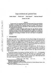
Figure 2. Numerical evaluation of L1 ψQ (s) for the Simple Exclusion Process (N = 200, L = 400). (a: Left) Comparison between direct numerical measurement (blue crosses) and result from thermodynamic integration (red circles). (b: Right) Comparison between numerical results (red circles) and analytical prediction (22) valid for small s (blue line).

As in other exclusion processes [9, 13], the large deviation function ψQ (s) is extensive in the system size and we rather study the rescaled large deviation function 1 ψ (s) in the thermodynamic limit (N and L are large, the density ρ = N/L being L Q fixed). Though on average the total current is zero (the moves are symmetric), the variance is finite and ψQ (s) reads for small s [11, 21] 1 ψQ (s) = ρ(1 − ρ)s2 + O(Ls4 ) (22) L In this regime, the fluctuations are Gaussian and our algorithm yields results in perfect agreement with the expansion (22) (see Figure 2b). For larger values of s, we lack an analytic expression for ψQ (s) but the algorithm still applies successfully. We found non-Gaussian fluctuations (Figure 2a), which correspond to very large deviations of the current. The direct measurement of ψQ (s) is also compared with the results obtained from thermodynamic integration (Figure 2a). Both evaluations coincide within numerical accuracy, though the latter requires duration more than one order of magnitude smaller to converge. 3.2. The Asymmetric Simple Exclusion Process (ASEP) We now consider the large deviations of the total current Q in a non-equilibrium system, the Asymmetric Simple Exclusion Process [21] with closed boundary conditions. The

A numerical approach to large deviations in continuous-time

8

4000 2000 0 -10

-6

-2

2

6

10

s Figure 3. Plot of the large deviation function L1 ψQ (s) of the Asymmetric Simple Exclusion Process, for L = 400 sites and N = 200 particles. The jump rates are p = 1.2 and q = 0.8, whence E ≃ −0.2. Blue crosses and red circles correspond to direct computation and thermodynamic integration respectively. The asymmetry appears when comparing the extreme points s = ±9.5.

ρ

1

1

0.8

0.8 n

0.6

0.6

0.4

0.4

0.2

0.2

0

0

25

50 position

75

100

0

0

25

50 position

75

100

Figure 4. (a: Left) Average profile ρ for s = 0.3. To minimise the overall current, the system develops an asymmetric shock, where only the front particles can jump easily. (b: Right) A typical configuration for |s| ≫ E. The particles are distributed almost uniformly.

system is composed of N particles diffusing on a one-dimensional lattice of size L. Each particle can jump with rate p to its left and q to its right, provided the arrival site is empty. The total current Q is defined as in the previous section. For p 6= q, a non-zero steady current flows through the system. We report in Figure 3 the large deviation function ψQ (s). One notes the symmetry around E = 12 ln pq , guaranteed by the fluctuation theorem. The histories which contribute to ψQ (s) around s ≈ E (Q ≈ 0) clearly display shocks (Figure 4a) while a large current (|s| ≫ E) is provided by uniform profiles (Figure 4b).

4

1.2

3

0.8

′ (s) ψK L

ψK (s) L

A numerical approach to large deviations in continuous-time

2

9

0.4

1 0 -1.5

0 -0.5

0.5

1.5

s

0

0.04

0.08

0.12

s

Figure 5. (a: Left) Plot of the large deviation function L1 ψK (s) associated to the number of events K in the Contact Process in a field (L = 120 sites) (b: Right) The dynamical phase transition occurs at sc ∼ 0.057. This is exemplified by plotting ′ ψK (s) = 1t hKis for different system sizes (L = 4 in black, 8 in red, 15 in blue and 50 in magenta)

3.3. The Contact Process (CP) We now turn our attention to the Contact Process [23] in one dimension. The model is defined on a lattice of L sites with periodic boundary conditions. Each site i is either empty (ni = 0) or occupied by a particle (ni = 1). The dynamics is defined as follows: particles annihilate with rate 1, while empty sites i get occupied with rate W (ni = 0 → ni = 1) = λ(ni−1 + ni+1 ) + h

(23)

where λ and h are positive constants. Note the presence of a spontaneous rate of creation h. When h = 0, the systems always reaches an absorbing empty state in finite size [24, 25], while the steady state is active for λ > 1 in the thermodynamic limit. On the contrary, the addition of a small field h leads to an active equilibrium state for all λ. In the mean field version, the equilibrium dynamics is still influenced by the presence of an inactive state. This can be seen through the study of the large deviations of the number of events K, a quantity which simply counts the number of configuration changes during an history of the system. It was proved that L1 ψK (s) is non-analytic at a critical value sc , which goes to zero with h. As pointed out in section 2.2 the large deviation function ψK (s) plays the role of a dynamical free energy, whose nonanalyticities are synonymous of dynamical phase transitions. In physical terms, this corresponds to the existence of two distinct classes of histories [19]: the active phase dominates the steady state, while large deviations corresponding to s > sc are dominated by inactive histories. For s = sc , the two phases coexist in a first-order fashion. The question whether this transition is still present in finite dimension is still open. Using our algorithm, we obtain evidence that this is indeed the case in dimension 1. In Figure 5a, we plot the function ψK (s) for a large system size and for values of the parameters λ = 3.5, h = 0.1. The two branches of the function correspond to

A numerical approach to large deviations in continuous-time

10

the two dynamical phases mentioned above. As in the mean field version, the nonanalycity appears as a jump in the first derivative of L1 ψK (s) in the thermodynamic ′ limit. Using the relation ψK (s) = − 1t K s (see section 2.4), we can study the finite size ′ scaling of L1 ψK (s) (Figure 5). The results support the presence of a phase transition at sc ∼ 0.057. Around sc , the dynamics presents a superposition of “more active” and “less active” histories, for which the continuous-time approach is particularly helpful. 4. Conclusions We have presented a simple algorithm to evaluate large deviation functions in continuous-time Markov chains without relying on any time discretisation. We have shown on specific examples that the method can be used successfully in systems where the presence of different time scales renders the discrete-time approach difficult. In the context of quantum simulations, an approach to continuous-time versions of Diffusion Monte Carlo was proposed by Sylju˚ asen [26], using a continuous formalism but a discrete time implementation. One can expect that the algorithm we have introduced could also be interesting in such context. Acknowledgments This work has been supported in part by the French Ministry of Education through the Agence Nationale de la Recherche’s programme JCJC/CHEF (VL). VL gratefully acknowledges the warm hospitality at the Laboratoire de Physique et M´ecanique des Milieux H´et´erog`enes, ESPCI, Paris, France, where part of this work was completed. We thank Christian Giardin`a, Jorge Kurchan, Paolo Visco and Fr´ed´eric van Wijland for useful discussions. Appendix A. An explicit formula for Z(s, t) can be written as the sum over C of the solution of (14):

Z(s, t) =

X

X

K≥0 C1 ,...,CK−1 ,C

Y(C0 )t1 −t0

Z

0

t

dµstK

Z

0

tK

dµstK−1

...

Z

t2 0

dµst1 e−(t−tK )rs (C)

(A.1)

Ws (CK−1 → C) Ws (C0 → C1 ) . . . Y(CK−1)tK −tK−1 Y(C)t−tK rs (C0 ) rs (CK−1 )

where rs (C) =

X

Ws (C → C ′ )

(A.2)

C ′ 6=C

is the escape rate from the configuration C in the s-modified dynamics, dµstk = dtk rs (Ck ) exp[−(tk − tk−1 )rs (Ck )]

(A.3)

A numerical approach to large deviations in continuous-time

11

represents the probability of the time intervals between jumps, and Y(Ck )tk+1 −tk = e(tk+1 −tk )(rs (Ck )−r(Ck )) (A.4) is the exponential increase of Pˆ between tk and tk+1 . We can read in this formula the direct expression of the cloning factors used at the step (3) of the algorithm. References [1] Giardin`a C, Kurchan J, and Peliti L, Direct Evaluation of Large-Deviation Functions, Phys. Rev. Lett. 96 120603 (2006), ¨ [2] Einstein A, Uber die von der molekularkinetischen Theorie der W¨arme geforderte Bewegung von in ruhenden Fl¨ ussigkeiten suspendierten Teilchen, Ann. d. Phys. 17 549 (1905) [3] Ellis R S, Entropy, large deviations, and Statistical Mechanics, (Springer-Verlag, New York, 1985) [4] Evans D J, Cohen E G D, and Morriss G P, Probability of second law violations in steady flows, Phys. Rev. Lett. 71 2401 (1993) [5] Gallavotti G and Cohen E G D, Dynamical ensembles in nonequilibrium statistical mechanics, Phys. Rev. Lett. 74 2694 (1995) [6] Jarzynski C, Nonequilibrium equality for free energy differences, Phys. Rev. Lett. 78 2690 (1997) [7] Kurchan J, Fluctuation theorem for stochastic dynamics, J. Phys. A: Math. Gen. 31 3719 (1998) [8] Crooks G E, Nonequilibrium Measurements of Free Energy Differences for Microscopically Reversible Markovian Systems, J. Stat. Phys. 90 1481 (1998) [9] Lebowitz J L and Spohn H, A Gallavotti-Cohen type symmetry in the large deviation functional for stochastic dynamics, J. Stat. Phys. 95 333 (1999) [10] Ciliberto S and Laroche C, J. Physique IV 8 Pr6-215 (1998); Wang G M, Sevick E M, Mittag E, Searles D J, and Evans D J, Phys. Rev. Lett. 89 050601 (2002); Bustamante C, Liphardt J, and Ritort F, Physics Today 58, 43 (2005); Ritort F, in Poincar´e Seminar 2, 195 (Birkh¨ auser: Basel, 2003); [11] Bodineau T and Derrida B, Current fluctuations in non-equilibrium diffusive systems: an additivity principle, Phys. Rev. Lett. 92 180601 (2004) ; [12] Bertini L, De Sole A, Gabrielli D, Jona-Lasinio G, and Landim C, Current fluctuations in stochastic lattice gases, Phys. Rev. Lett. 94 030601 (2005) ; [13] Derrida B and Lebowitz J L, Exact large deviation function in the asymmetric exclusion process, Phys. Rev. Lett. 80 209 (1998) ; [14] Ruelle D, Thermodynamic Formalism, 1978, Addison-Wesley, Reading (Mass.). [15] Grassberger P, Go with the winners: a general Monte Carlo strategy Comp. Phys. Comm. 147 64-70 (2002 ) [16] Grassberger P, Badii R, and Politi A, Scaling laws for invariant measures on hyperbolic and nonhyperbolic attractors, J. Stat. Phys 51, 135 (1988) 135 - 178 [17] Tailleur J, Kurchan J, Probing rare physical trajectories with Lyapunov weighted dynamics, e-print cond-mat/0611672, to appear in Nature Physics [18] Gaspard P, Chaos, scattering and statistical mechanics (CUP, Cambridge, 1998). [19] Lecomte V, Appert-Rolland C, and van Wijland F, Thermodynamic formalism for systems with Markov dynamics, e-print cond-mat/0606211, to appear in J. Stat. Phys. [20] Anderson J B, A random-walk simulation of the Schr¨odinger equation: H3+ , J. Chem. Phys. 63 1499 (1975) [21] Spohn H, Long range correlations for stochastic gases in a non-equilibrium steady state, J. Phys. A: Math. Gen. , 16 4275 (1983) [22] Spohn H, Large scale dynamics of interacting particles, (New York, Springer, 1991) [23] Harris T E, Contact Interactions on a Lattice, Ann. Probab. 2 969 (1974) [24] Dickman R and Vidigal R, Quasi-stationary distributions for stochastic processes with an absorbing state, J. Phys. A: Math. Gen. 35 1147 (2002)

A numerical approach to large deviations in continuous-time

12

[25] Deroulers C and Monasson R, Field theoretic approach to metastability in the contact process, Phys. Rev. E 69 016126 (2004) [26] Sylju˚ asen O F, Continuous-time diffusion Monte Carlo and the quantum dimer model, Phys. Rev. B 71 020401 (2005)