A Large Deviations Approach to Statistical Traffic Anomaly Detection∗ Ioannis Ch. Paschalidis†
Abstract— We introduce an Internet traffic anomaly detection mechanism based on large deviations asymptotic results. Using past traffic traces we characterize network traffic during various time-of-day intervals, assuming that it is anomaly-free. We present two different approaches to characterize traffic: (i) a model-free approach based on the method of types and Sanov’s theorem, and (ii) a model-based approach modeling traffic using a Markov modulated process. Using these characterizations as a reference we continuously monitor traffic and employ large deviations results to compute the probability that the monitored traffic is “consistent” with the corresponding reference characterization. Low values of this probability identify, in real-time, traffic anomalies. Our experimental results show that applying our methodology (even short-lived) anomalies are identified within a small number of observations. Throughout, we compare the two approaches presenting their advantages and disadvantages. We validate our techniques by analyzing real traffic traces with time-stamped anomalies. Index Terms— Network security, intrusion detection, statistical anomaly detection, method of types, large deviations.
I. I NTRODUCTION LTHOUGH significant progress has been made in network monitoring instrumentation, automated on-line traffic anomaly detection is still a missing component of modern network security and traffic engineering mechanisms. Previous studies showed that many types of traffic anomalies, such as attacks, worms, misconfiguration, network failures and a rapid increase of traffic volume (flash crowds), can be detected by monitoring the aggregate traffic at a border router. These approaches are typically grouped in two categories: signature based anomaly detection where known patterns of past anomalies are used to identify ongoing anomalies [1, 2], and statistical anomaly detection which identifies patterns that substantially deviate from normal patterns of operation [3]. Recent research studies showed that systems based on pattern matching had detection rates below 70% [4]. Furthermore, such systems need constant (and expensive) updating to keep up with new attack signatures. As a result, more attention has to be drawn to statistical methods for traffic anomaly detection since they can identify even novel (unseen) types of anomalies. In this paper we introduce a new statistical traffic anomaly detection framework that employs rigorous fault detection methodologies at short time scales. Our approach is fairly
A
* Research partially supported by the NSF under grants DMI-0330171, DMI-0300359, CNS-0435312, ECS-0426453 and by the ARO under the ODDR&E MURI2001 Program Grant DAAD19-01-1-0465 to the Center for Networked Communicating Control Systems. † Corresponding author. Center for Information & Systems Eng., and Dept. of Manufacturing Eng., Boston University, 15 St. Mary’s St., Brookline, MA 02446, e-mail:
[email protected], url: http://ionia.bu.edu/. ‡ Computer Science Department, Boston University, e-mail:
[email protected].
Georgios Smaragdakis‡
standard for statistical anomaly detection. First, we learn what constitutes “normal behavior” by observing past system behavior, assuming that it is anomaly-free. Using this knowledge we continuously monitor the system to identify time instances where system behavior does not appear to be normal. The novelty of our approach is in the way we characterize normal behavior and in how we assess deviations from it. More specifically, we propose two methods to characterize normal behavior: (i) a model-free approach employing the method of types [5] to characterize the type (i.e., empirical measure) of an i.i.d. sequence of appropriately averaged system activity, and (ii) a model-based approach where system activity is modeled using a Markov Modulated Process (MMP). Given these characterizations of normal behavior obtained from past system history, we compute the probability that current system behavior deviates from normal. Naturally, we employ the theory of Large Deviations (LD) [5]. LD theory provides a powerful way of handling rare events and their associated probabilities. The two key technical results we rely upon are Sanov’s theorem [5] in the model-free approach and a related result for the empirical measure of a Markov process for the model-based case. We note that the words “traffic” and “router” are purposefully absent from the previous paragraph. Rather, we use the generic term “system”. This is to indicate that our approach can be easily adapted to identify anomalies in any trace of system activity we would like to monitor (e.g., access to various application ports, IP source-destination addresses, system calls, etc.). In this paper, however, we focus on two case studies: (a) three different representations (bytes, packets and flows) of sampled origin-destination flow data from a backbone network, and (b) the aggregate traffic that arrives to or originates from the border router of some local area network (LAN) we wish to monitor. Traffic has diurnal variations which are primarily due to human activity. However, for relatively short time-scales (e.g., of about an hour), and especially during busy hours, stationary models can be appropriate [6]. The model-free approach aggregates traffic over short time intervals to which we will refer to as time buckets. Although the correlation between samples in short time scales is significant, it reduces rapidly between aggregates over a time bucket. Hence, we consider the sequence of traffic aggregates over a bucket as an i.i.d. sequence and employ the method of types to characterize its distribution. Our model-based approach uses an MMP process to model legitimate traffic during some time-of-day interval. Earlier work has shown that MMP models can accurately characterize network traffic [7, 8]. The methods we present are statistical; as a result, our approach has the potential of detecting novel anomalies, such as previously unseen attacks. This is crucial for network security as new types of attacks are constantly being engineered. A novel feature of our approach is that it compares subtle distributional differences between the
reference traffic characterization and observed traffic traces. As we will see, this is critical as it enables us to detect attacks –including some short-lived ones– that do not result in significant changes in traffic volume. First or second moments of traffic measurements would be too insensitive to these types of attacks. To the best of our knowledge, this is the first attempt to develop a framework that provides a statistical on-line methodology for anomaly detection in short time scales identifying temporal anomalies as opposed to techniques working over much longer time-scales [3]. The only infrastructure requirement in order to deploy our method is a simple counter. As mentioned earlier, we rely upon observing the system during an anomaly-free period to learn what constitutes normal behavior. Of course, one can never ensure that a trace of system activity is anomaly-free. Yet, even in those cases that the reference trace is “tainted” it is useful to know that the current activity is statistically different. Moreover, one would often update the reference trace with more recent activity, thus, almost eliminating the possibility that non-typical behavior (hence, relatively short-lived) will be classified as typical. We report a number of experimental results from applying our approaches to two different network traces: (a) one week of sampled origin-destination flow data from the Abilene backbone network, and (b) the 1999 MIT Lincoln Lab (DARPA evaluation) trace [4]. We are able to detect a variety of anomalies such as attacks and volume anomalies (even short ones) within a few samples, with very high success rate and low false alarm rate. The rest of the paper is organized as follows. In Section II we present our model-free method for anomaly detection. In Section III, we provide the basic theoretical background of our model-based method. In Sections IV and V we compare the two methods and validate our methodology using real measurements with time-stamped anomalies. In Section VI we review related work and identify the major differences with our approaches. We conclude in Section VII.
where L (·) is the log-likelihood of the model with respect to a process realization. The key observation motivating the AIC is that L (·) tends to favor models with a larger number of free parameters. The AIC removes this bias by introducing a penalty for the number of free parameters; thus, the resulting N is considered the most appropriate for the given trace (minimizing modeling and estimation error). Once we have N , elements of the alphabet that are not observed in the trace are merged with neighboring ones to obtain N ′ which is the final size of the alphabet. A. Large Deviations of the Empirical Measure Combinatorial methods can be applied for∗ the empirical ∗ b measures of Σ-valued process. Let Yt = (Yt−w+1 , . . . , Ytb ) be the trace of the w most recent partial sums using a bucket size b∗ . We assume that these random variables are i.i.d., following a law µ ∈ M1 (Σ), where M1 (Σ) denotes the space of all probability measures on the alphabet Σ. Let also, Σµ denote the support of µ, i.e., Σµ = {αi : µ(αi ) > 0}. Define the type (empirical measure) of Yt as Yt Ew,b ∗ (αi ) =
Q(N, r1 , . . . , rN −1 ) = −L (r1 , . . . , rN −1 ) + N (N − 1),
i = 1, . . . , N, ∗
b being of type where 1αi is the indicator function of Yt−w+j Yt αi . Namely, Ew,b∗ (αi ) is the fraction of occurrences of αi in Yt Yt t the sequence Yt . Let E Y w,b∗ = (Ew,b∗ (α1 ), . . . , Ew,b∗ (αN )). The next theorem, which is due to Sanov, establishes a t large deviations result for E Y w,b∗ (see [5, Sec. 2.1.10]).
Theorem II.1 For every ν ∈ M1 (Σ) let I1 (ν) = H(ν|µ), where H(ν|µ) is the relative entropy of the probability vector ν with respect to µ: △
H(ν|µ) =
II. A M ODEL -F REE A PPROACH In this section we discuss our model-free approach. Consider a time series X1 , . . . , Xn of traffic activity (say, in bits/bytes/packets/flows per sample). Let Ytb the partial sum (or aggregate traffic) over the time bucket starting Pb at (t − 1)b and containing b samples, namely, Ytb = i=1 X(t−1)b+i . ∗ b∗ The crucial assumption we make is that Y1b , . . . , Y⌊n/b⌋ is an i.i.d. sequence for some appropriate bucket size b∗ . (It is possible to select such a b∗ by finding the value of b∗ so that |ACF (k)| ≤ √2n , ∀ k > b∗ , where ACF (k) = E[(Xt − µ)(Xt+k − µ)]/σ 2 is the autocorrelation function with µ denoting the mean and σ 2 the variance of the timeseries.) ∗ We quantize the values of the partial sums Ytb mapping them to the finite set Σ = {α1 , . . . , αN } of cardinality N . For the rest of the paper, we will be referring to Σ as the underlying alphabet. The quantization is done as follows: we ∗ let [r0 , rN ] the range of values Ytb takes, divide it into N subintervals [r0 , r1 ], . . . , [rN −1 , rN ] of equal length, and map [ri−1 , ri ] to αi for i = 1, . . . , N . To select the appropriate size of the alphabet N we follow the approach of [8] and use the so called Akaike’s Information Criterion (AIC) [9]. In particular, N is set to minimize:
w ∗ 1 X ), 1α (Y b w j=1 i t−w+j
N X
ν(αi ) log
i=1
ν(αi ) . µ(αi )
Then, for any set Γ of probability vectors in M1 (Σ) − inf◦ I1 (ν) ≤ lim inf
w→∞
ν∈Γ
1 t EY log P[E w,b∗ ∈ Γ] w
1 t EY log P[E inf I1 (ν), w,b∗ ∈ Γ] ≤ − ν∈Γ w→∞ w
≤ lim sup
where Γ◦ denotes the interior of Γ. More intuitively, Theorem II.1 states that for a long trace Yt (i.e., large w) its empirical measure is “close to” ν with probability that behaves as −wI1 (ν) t EY P[E . w,b∗ ≈ ν] ∼ e
B. Anomaly Detection Algorithm Theorem II.1 can be used to identify anomalies. The proposed algorithm is summarized as follows: 1) From an anomaly-free trace construct the alphabet Σ = {α1 , . . . , αN } and the empirical measure (law) µ induced by this sequence. ∗ b∗ , . . . , Ytb ) be 2) For each time t let Yt = (Yt−w+1 the trace of the w most recent partial sums using a
bucket size b∗ . Compute its empirical measure and let t EY w,b∗ = ν t,w be the result. △
3) Then, ρt,w = e−wI1 (ν t,w ) approximates the probability that the trace Yt is drawn from the probability law µ. If ρt,w is consistently low over some observed time interval, we can conclude that the observed trace deviates from the anomaly-free trace, which indicates an anomaly. ρt,w can be better observed in the logarithmic scale. Formally, we identify an anomaly at time t if ρτ,w < ǫ,
∀τ = t − k + 1, . . . , t,
(1)
where n is the length of the traffic trace we process, w = ⌊n/b∗ ⌋ is the number of partial sums we generate from this trace, and ǫ is the detection threshold we use. The parameters n, b∗ , k, ǫ affect the rule’s performance and can be tuned experimentally. Notice that we can compute consecutive ρτ,w by using a sliding window of length n. Thus, we generate a new value for ρτ,w with every traffic sample. As we will see, this enables us to detect anomalies very fast. We proceed by presenting a model-based method, where the i.i.d assumption is not a requirement, thus it can be directly applied to the timeseries and not to the partial sums. III. A M ODEL -BASED A PPROACH We start with devising an MMP model for representing traffic activity. We should point out that our goal is not to adopt the most sophisticated and accurate traffic model; the quality of the model should be judged based on whether it is useful in anomaly detection. A. An MMP model We assume that the origin-destination traffic (in bits/bytes/packets/flows per time unit) or the (inbound or outbound) traffic trace observed at a border router, corresponding to a specific time-of-day interval, can be characterized by a stationary model over a certain period (e.g., a month) if no technological changes (e.g., link bandwidth upgrades) have taken place. A traffic trace can be a sequence of bits/bytes/packets/flows per time unit, where time units are defined depending on the available data or as we see fit for detecting anomalies. We propose the use of an MMP to model the traffic activity during a small time interval (several hours). Such a process is characterized by an underlying Markov chain with transition probability matrix Ξ. To each state i, i = 1, . . . , M , we associate an interval [ri−1 , ri ] of real numbers from which observations are drawn. That is, when the MMP is in state i traffic activity observations range in [ri−1 , ri ]. (For the application we are considering we do need to specify how observations are drawn from [ri−1 , ri ]; in general they can follow some probability distribution.) MMPs, when the state is “hidden”, are also known in the literature as Hidden Markov Models (HMMs) [10]. We restrict ourselves to models in which the ranges of possible observations corresponding to different states are disjoint. Thus, an observation can be uniquely associated to an MMP state (the state is no longer hidden) and therefore the term disjoint Markov Modulated Process (d-MMP) is more appropriate. To model the traffic trace as a d-MMP we let [r0 , rM ] be the the range of all observations we make, split [r0 , rM ] into M subintervals of equal length, and assign state i, i = 1, . . . , M , to interval [ri−1 , ri ]. To select the appropriate
number of states M we use the AIC as in Section II. Given M , the transition probabilities Ξ are obtained via maximum likelihood estimation. We consider the constructed model to be reliable since it is the outcome of a long period of anomaly-free observations. Different models can be constructed for different time-of-day intervals (business hours, evening hours, overnight, etc.). B. Large Deviations of the Empirical Measure Once we obtain the d-MMP model from an anomaly-free trace we are interested in comparing ongoing traffic activity to the model in order to identify potential deviations that would indicate an anomaly. To that end, given any trace we need to determine the probability that the trace is “explained” by the model. Assume that the d-MMP has an irreducible underlying Markov chain with M states 1, 2, . . . , M and transition probability matrix Ξ = {p(i, j)}M i,j=1 . Let p denote the vector consisting of the rows of Ξ. Let Y denote a sequence Y1 , Y2 , . . . , Yn of states that the Markov chain visits with the initial state being Y0 = σ, and consider the empirical measures n 1X Y 1y (Yk−1 Yk ), En,2 (y) = n k=1
2 △
where y ∈ A = {1, . . . , M } × {1, . . . , M } and 1y is the indicator function for the subset y. Note that when Y y = (i, j) ∈ A 2 the empirical measure En,2 (y) denotes the fraction of times that the Markov chain makes transitions △ from i to j in the sequence Y. Let now Ap2 = {(i, j) ∈ 2 A | p(i, j) > 0} denote the set of pairs of states that can appear in the sequence Y1 , Y2 , . . . , Yn and denote by M1 (Ap2 ) the standard |Ap2 |-dimensional probability simplex, where |Ap2 | denotes the cardinality of Ap2 . Note that the Y Y 2 vector of En,2 (y)’s, denoted by E Y n,2 = (En,2 (y); y ∈ Ap ), is an element of M1 (Ap2 ). For any q ∈ M1 (Ap2 ), let △
q1 (i) =
M X
q(i, j)
and
△
q2 (i) =
M X
q(j, i)
(2)
j=1
j=1
△
be its marginals. Whenever q1 (i) > 0, let qf (j | i) = q(i, j)/q1 (i). We will be using the notation qf = (qf (1 | 1), . . . , qf (M | 1), qf (1 | 2), . . . , qf (M | M )). We say that a probability measure q ∈ M1 (Ap2 ) is shift invariant if both its marginals are identical, i.e., q1 (i) = q2 (i) for all i. A large deviations result for E Y n,2 is established in the next theorem and is proven in [5, Sec. 3.1.3]. Theorem III.1 ([5]) For every q ∈ M1 (Ap2 ) let M X q1 (i)H(qf (· | i) | p(i, ·)), if q is shift I2 (q) = i=1 invariant, ∞, otherwise,
where H(qf (· | i) | p(i, ·)) is the relative entropy, that is, H(qf (· | i) | p(i, ·)) =
M X j=1
qf (j | i) log
qf (j | i) . p(i, j)
Then, for any set Γ of probability vectors in M1 (Ap2 ), − inf◦ I2 (q) ≤ lim inf
n→∞
q∈Γ
1 EY log P[E n,2 ∈ Γ] ≤ n
1 EY log P[E n,2 ∈ Γ] ≤ − inf I2 (q), q∈Γ n n→∞
lim sup
where Γ◦ denotes the interior of Γ. More intuitively, Theorem III.1 states that for a long trace Y (i.e., large n) its empirical measure is “close to” q with probability that behaves as −nI2 (q) EY P[E . n,2 ≈ q] ∼ e
C. Anomaly detection algorithm Theorem III.1 can be used to identify anomalies. The proposed algorithm is summarized as follows. 1) From an anomaly-free trace obtain a d-MMP as outlined in Subsection III-A. Let p be the resulting transition probability vector. 2) For each time t let Yt = (Yt−n+1 , . . . , Yt ) be the trace of current traffic activity consisting of n consecutive traffic measurements. Compute its empirical measure t and let E Y n,2 = qt,n be the result. △
3) Then, ρt,n = e−nI2 (qt,n ) approximates the probability that the trace Yt is drawn from the d-MMP with transition probability vector p. If ρt,n is consistently low over some observed time interval, we conclude that the observed trace is not “consistent” with the reliable model, which indicates an anomaly. As we will see, ρt,n can be better observed in a logarithmic scale. For an automated anomaly detection rule one can use the rule in 1, i.e., identify an anomaly at time t if ρτ,n < ǫ,
∀τ = t − k + 1, . . . , t,
(3)
where n, k and ǫ are the parameters affecting the rule’s performance (success and false alarm rates) and which have to be tuned. Obviously, other variations of this rule are possible, for instance, setting a threshold for the time-average of ρτ,n over the window [t − k + 1, . . . , t]. IV. E XPERIMENTAL S ETUP I: T HE A BILENE DATA S ET In this section, we validate our methodology against real traffic from a backbone network. Our source of data is the IPlevel traffic flow measurements collected form every point of presence (PoPs) in the Abilene Internet2 backbone network. Abilene is the major academic network, connecting over 200 universities in the US, and peering with other research networks in Europe and Asia. Abilene has 11 PoPs resulting in 121 origin-destination flows. The data we are using is sampled flow data from every router of Abilene for a period of one week (April 7 to 13, 2003). Sampling is random capturing of 1% of all packets entering every router. Three different representations (features) of sampled flow data are used, as timeseries of the number of bytes (B), of packets (P) and of flows (F). In order to avoid synchronization issues, the measurements are aggregated into 5 minutes bins. A log with the anomalies that took place is also provided. Three different types of anomalies are present: DoS: distributed Denial of service attack against a single victim; SCAN : scanning a host for a vulnerable port (port scan)
or scanning the network for a target port (network scan); AP LHA: unusually high rate point to point byte transfer. There are also some anomalies that are labeled as unknown (U N KN ). In total there are 271 anomalies: 133 DoS, 81 SCAN, 32 ALPHA and the rest are unknown [11]. Origin-destination flows aggregate the traffic of thousands of connections (in a period of 5 minutes), thus, traffic anomalies of a destination may hide in the byte representation, but can appear in other representations like the packet or flow representations. DoS anomalies were always present in the packet (P) representation. This is expected as most DoS attacks bombard a single destination with a huge number of packets. Instances of DoS are not observed in the flow representation and may be observed in the byte (B) representation. The SCAN anomalies are observed only in the flow (F) representation. ALPHA anomalies are characterized by spikes in the byte representation only. Following the above observations we can even characterize anomalies that are denoted as unknown. A. Outline of the Technique We apply both our methods to the different timeseries (representations of B/P/F) for the 121 origin-destination flows. In order to avoid the effect of diurnal variation we consider 200 samples (each one representing the activity of 5 minutes) every day. We use as reference the activity that has been observed for the same time interval the previous day. For the first day of the week, as we do not have information from the previous day, we take as reference the network activity of the second day. We apply the model-free approach following the algorithm described in Subsection II-B. We construct the alphabet of the three representations and the corresponding probability law for every day of the anomaly-free week. We then process the network activity for the next day. We compute ρt,w – the probability that the observed traffic follows the same (anomaly-free) law – using the procedure outlined in Subsection II-B. Working with statistics of the autocorrelation function, we found that b∗ = 3 and w = 10 are good values for our data set. In order to identify the threshold ǫ in (1) we run our algorithm and compute ρt,w for the reference trace, which should yield O(1) probabilities. We found that ρt,w is always below 10−3 in the reference trace, thus we set ǫ = 10−3 . We also follow the approach of Section III-A to devise an appropriate d-MMP traffic model. Using this model, for every day of the week and for every time sample we compute ρt,n – the probability that the observed traffic trace is consistent with the d-MMP model – for an appropriately selected trace length n (cf. Step 2 of the algorithm in Subsection III-C). By following the same procedure as above, we select ǫ = 10−2 in (3). On a notational remark, we denote an anomaly as ORIGDEST-xxxx, where ORIG is the ingress PoP, DEST is the egress PoP and xxxx is the time point in the time series (from 1 − 2016) of the related representation where an anomaly occurs. B. Anomaly Detection Examples In this subsection we discuss the performance of our framework and we compare the two proposed methods. Fig. 1, illustrates a DoS attack in the Indianapolis-Seattle origin-destination flow and the associated probability ρt,w
4
4
3
2
1
0
10
20
30
40
50
60
70
80
90
WASH−NYCM−610
0
10
3
Threshold
−5
10
−2
10
Threshold
2 1.5 1
−10
0
10
20
30
40
50
60
70
80
90
10
100
−4
0
10
20
30
40
50
60
70
80
90
10
100
0
0
10
STTL−NYCM−173
0
10
2.5
100
0
IPLS−STTL−1069
x 10
3.5
ρ
packets every 5 minutes
packets every 5 minutes
IPLS−STLTL−1069
x 10
ρ
4
4
10
20
30
40
50
60
70
80
90
100
30
40
50 samples
60
70
80
90
100
0
10
10
0
10
−1
10
−1
10
−2
ρ
Threshold
ρ
ρ
ρ
Threshold
−3
10
Threshold
−1
10
−2
10 −2
10
Threshold
−2
10
10
−4
10 −4
10
−3
−5
10
0
10
20
30
40
50 samples
60
70
80
90
100
Fig. 1. Model-Free Method. (Top): Packet representation for the Indianapolis-Seattle flow. (Bottom): Value of ρt,w . The rectangle denotes a DoS attack.
0
10
20
30
40
50 samples
60
70
80
90
100
Fig. 2. Model-Based Method. (Top): Packet representation for the Indianapolis-Seattle flow. (Bottom): Value of ρt,n . The rectangle denotes a DoS anomaly.
when the model-free based method is applied. This probability is significantly low in the vicinity of the anomaly. It is to be expected that it can not pinpoint the time of the anomaly due to aggregation effect of the partial sums and our use of a window of size w. In the absence of any information on when the anomaly occurs within this window we can estimate its time as w2 time units after the first time ρt,w drops below ǫ. On the other hand, applying the modelbased method (Fig. 2), we can more precisely identify when an anomaly occurs. The disadvantage of the model-based method is that the false alarm rate is larger than that of the model-free method which benefits from the averaging over the time bucket b∗ . The same observations are valid for other types of attacks, namely SCAN (Fig. 3) and ALPHA (Fig. 4). We summarize our results in Table I. We should point out that the performance of our framework is related to the sampling frequency, i.e., if we increase the sampling frequency to 1 minute or even few seconds, we expect the sensitivity of our detection mechanism (and hence, the success rate) to increase. V. E XPERIMENTAL S ETUP II: T HE DARPA E VALUATION DATA S ET Next, we validate our method against the 1999 MIT Lincoln Lab (DARPA Evaluation) data set [4]. The data set consists of tcpdump data collected at the border router of a local network. Three weeks of training data were provided in the DARPA Evaluation data set. The first and third weeks of the training data do not contain any attacks. This data was provided to facilitate the training of anomaly detection systems. The second week of the training data contains a selected subset of attacks from the 1998 DARPA evaluation data set in addition to several new attacks. In addition, two weeks of network based attacks in the midst of normal background data were also provided. The experimental setting includes different types of machines and operating systems. There are 201 instances of about 56 types of attacks distributed throughout these two weeks. In particular, the attack events that either occurred or were attempted are the following: Denial of Service (DoS) –unauthorized attempt to disrupt the normal functioning of a victim host or network; Remote to Local (R2L) –obtaining user privileges on a local host by a remote user without proper authorization; User to Root (U2R) –unauthorized access to local superuser or administrator privileges by a local unprivileged user; Surveillance or Probe (PROBE) –unauthorized probing of a machine or network to look for vulnerabilities, explore configurations, or map the network’s topology; and Data
10
−3
0
10
20
30
40
50 samples
60
70
80
90
100
Fig. 3. Comparison of the two methods. (Top): Model-Free Method, (Bottom): Model-Based Method. The rectangle denotes a SCAN anomaly.
10
0
10
20
Fig. 4. Comparison of methods. (Top): Model-Free (Bottom): Model-Based The rectangle denotes an anomaly.
the two Method, Method. ALPHA
Compromise (DATA) –unauthorized access or modification of data on a local or remote host. A detailed taxonomy of the attacks is presented in [12]. Throughout our study, we also observed some anomalies that we could not classify using the DARPA Evaluation report. Trying to classify these anomalies, we found that some of them are correlated with unusually high traffic volume; hence, we will refer to them as volume traffic anomalies. The identification of these types of anomalies is very important for traffic engineering tasks such as network provisioning, monitoring, pricing and mitigation of high traffic volume. A detailed study including these types of anomalies appeared in [11] showing their significance. We followed the same outline that was presented for the previous data set from Abilene. The first 36, 000 seconds (from 08:00-18:00) of the outbound traffic of each day of the first week were used to construct the alphabet and the d-MMP for the model-free and model-based model, respectively. We then observed the traffic of each day of the fifth week and we investigated how this deviates from the reference traffic of the same day of the first week. For the model-free method, the optimal values were found to be b∗ = 20, w = 3, k = 10 and the threshold was set to 10−3 . For the model-based method optimal the optimal values were n = 60, k = 3 and the threshold was set to 10−5 . The performance of both methods when applied to the DARPA data set is summarized in Table II. As there are no representations of different features in this data set, we give the aggregate false alarm rate for each method. VI. R ELATED W ORK In [3], the authors used wavelet filters to detect anomalies in network traffic including outages, flash crowds, attacks and measurements failures. Our approach differs from that one in the sense that we try to detect short-lived network traffic anomalies within a few samples. Namely, our method, as we implemented it, does not investigate traffic anomalies occurring over long time-scales (hours or days); instead we focused on anomalies over relatively short time-scales. Recently, a number of intrusion detection tools such as Snort [1] or Bro [2] have been developed. Their aim is to identify application specific intrusions and attacks. Our approach is clearly advantageous as it is not application specific and can identify most types of traffic anomalies. From a theoretical point of view, the authors in [13] studied a number of information-theoretic measures for anomaly detection. Their study was also performed using the DARPA Evaluation data set. Among other observations, they concluded that the relative entropy can better measure
Model-Free Method Anomaly
Model-Based Method
Success Rate
False Alarm Rate
Success Rate
False Alarm Rate
DoS
92%
5%
87%
10%
SCAN
92%
9%
86%
11%
ALPHA
93%
3%
87%
10%
UNKN
88%
10%
80%
12%
Overall
92%
7%
86%
11%
TABLE I S ETUP I: S UCCESS
AND FALSE ALARM RATES FOR EACH TYPE OF ANOMALY,
USING THE MODEL - FREE METHOD ( WITH ǫ1 AND
k = 3 SAMPLES ) AND
= 10−3 , w = 20, b∗ = 3 SAMPLES ,
THE MODEL - BASED METHOD ( WITH ǫ2
= 10−2 ,
n = 10 SAMPLES , AND k = 3 SAMPLES ). Model-Free Method
Model-Based Method
Success Rate
Success Rate
DATA
100%
100%
DoS
90%
86%
PROBE
89%
84%
R2L
86%
76%
U2R
88%
83%
Overall
90%
83%
7%
12%
Attack Category
False Alarm Rate
time interval. Using an anomaly-free trace it derives an associated probability law. Then it processes current traffic and computes the probability that it conforms to this probability law. The model-based method constructs a Markov modulated model of anomaly-free traffic measurements and relies on large deviations asymptotic results to compare this model to ongoing traffic activity. In particular, our results compute the probability that ongoing traffic activity is “consistent” with the model. In both methods, deviations in distributional characteristics of the traffic result in low values of the “conformance” probability, which identifies an anomaly. To the best of our knowledge, this is the first work for online anomaly detection based on large deviations results and distributional characteristics of empirical measures. We present a rigorous framework to identify traffic anomalies providing asymptotic thresholds for anomaly detection. We also estimate the size of the sliding window which provides reliable results for traffic anomaly detection in real-time. Since we monitor the detailed distributional characteristics of traffic and do not rely on the mean or the first few moments we are confident that our approach can be successful against new types of (emerging) attacks. Our method is of low implementation complexity (as it is based only on a counter), and is based on first principles, so it would be interesting to investigate how it can be embedded on routers or other network devices.
TABLE II S ETUP II: S UCCESS AND FALSE ALARM RATES FOR EACH TYPE OF = 10−3 , w = 3, ∗ b = 20 SECONDS AND k = 10 SECONDS ) AND THE MODEL - BASED METHOD ( WITH ǫ2 = 10−5 , n = 60 SECONDS , AND k = 10 SECONDS ).
ANOMALY, USING THE MODEL - FREE METHOD ( WITH ǫ1
the similarity between two datasets. Both our approaches rigorously derive a rule on how to compare two datasets. It turns out that the relative entropy plays a critical role in both rules we derive. The authors in [11, 14, 15] have introduced a framework to diagnose spatial anomalies, which is based on principal component analysis to partition the high dimensional space where a set of network traffic measurements live into disjoint subspaces corresponding to normal and anomalous conditions. Our methodology does not require whole network information and focuses on rapidly identifying temporal anomalies in each origin-destination flow or link. Very recently the authors in [15] used data mining and information theory techniques to identify network anomalies. Their methods take into account more information than the traffic volume, including, the origin and destination address of each flow, as well as source and destination ports using results from netflow. As we commented in the Introduction our methods can be easily adapted to handle such traces of activity as well. Our methods are on-line, providing a rigorous way to identify anomalies using a fixed sliding window. All the other methods we surveyed are off-line. VII. C ONCLUSIONS We introduced a general distributional fault detection scheme able to identify all sorts of temporal anomalies anomalies from attacks and intrusions to various volume anomalies and problems in network resource availability. We provided two different approaches, a model-free and a model-based one. The model-free method works on a longer time-scale processing traces of traffic aggregates over a small
Acknowledgments: We are grateful to Anukool Lakhina (Boston University) for providing us with the Abilene data set and for very helpful discussions. R EFERENCES [1] M. Roesch, “Snort - lightweight intrusion detection for networks,” in LISA ’99: Proceedings of the 13th USENIX conference on System administration, Seattle, Washington, November 1999, pp. 229–238. [2] V. Paxson, “Bro: a system for detecting network intruders in real-time,” Computer Networks, vol. 31, no. 23–24, pp. 2435–2463, 1999. [3] P. Barford, J. Kline, D. Plonka, and A. Ron, “A signal analysis of network traffic anomalies,” in Proceedings of the ACM SIGCOMM Workshop on Internet Measurement, Marseille, France, November 2002, pp. 71–82. [4] R. Lippmann, J. W. Haines, D. J. Fried, J. Korba, and K. Das, “The 1999 DARPA off-line intrusion detection evaluation,” Computer Networks, vol. 34, no. 4, pp. 579–595, 2000. [5] A. Dembo and O. Zeitouni, Large Deviations Techniques and Applications, 2nd ed. Springer-Verlag, New York, 1998. [6] M. Crovella, “Traffic modeling 101: Methods and results for single links and whole networks,” Tutorial presented at ACM SIGCOMM’04, Portland, OR, August 2004. [7] I. C. Paschalidis and S. Vassilaras, “On the Estimation of Buffer Overflow Probabilities from Measurements,” IEEE Transactions on Information Theory, vol. 47, no. 1, pp. 178–191, 2001. [8] ——, “Model-Based Estimation of Buffer Overflow Probabilities from Measurements,” in Proceedings of the ACM SIGMETRICS 2001/Performance 2001 conference, Cambridge, MA, June 2001, pp. 154–163. [9] H. Akaike, “Information theory and an extension of the maximum likelihood principle,” in 2nd International Symposium on Information Theory, Budapest, Hungary, 1973, pp. 267–281. [10] L. R. Rabiner, “A Tutorial on Hidden Markov Models and Selected Applications in Speech Recognition,” Proceedings of the IEEE, vol. 77, no. 2, pp. 257–285, February 1989. [11] A. Lakhina, M. Crovella, and C. Diot, “Characterization of NetworkWide Anomalies in Traffic Flows,” in Proceedings of the ACM SIGCOMM Internet Measurement Conference, Taormina, Italy, October 2004, pp. 201–206. [12] J. Mirkovic and P. Reiher, “A taxonomy of DDoS attack and DDoS defense mechanisms,” ACM SIGCOMM Compututer Communication Review, vol. 34, no. 2, pp. 39–53, 2004. [13] W. Lee and D. Xiang, “Information-theoretic measures for anomaly detection,” in Proceedings of the 2001 IEEE Symposium on Security and Privacy, May 2001, pp. 130–143. [14] A. Lakhina, M. Crovella, and C. Diot, “Diagnosing network-wide traffic anomalies,” in Proceedings of ACM SIGCOMM, Portland, OR, August 2004, pp. 219–230. [15] ——, “Mining Anomalies Using Traffic Feature Distributions,” in Proceedings of ACM SIGCOMM, Philadelphia, PA, August 2005, pp. 217 – 228.