Hindawi Mathematical Problems in Engineering Volume 2018, Article ID 1040476, 13 pages https://doi.org/10.1155/2018/1040476
Research Article A Numerical Computation Approach for the Optimal Control of ASP Flooding Based on Adaptive Strategies Shurong Li 1
1
and Yulei Ge
2
Automation School, Beijing University of Posts and Telecommunications, Beijing 100876, China College of Information and Control Engineering, China University of Petroleum (East China), Qingdao 266580, China
2
Correspondence should be addressed to Shurong Li;
[email protected] Received 12 December 2017; Revised 28 April 2018; Accepted 3 May 2018; Published 31 May 2018 Academic Editor: Łukasz Jankowski Copyright © 2018 Shurong Li and Yulei Ge. This is an open access article distributed under the Creative Commons Attribution License, which permits unrestricted use, distribution, and reproduction in any medium, provided the original work is properly cited. A numerical computation approach based on constraint aggregation and pseudospectral method is proposed to solve the optimal control of alkali/surfactant/polymer (ASP) flooding. At first, all path constraints are aggregated into one terminal condition by applying a Kreisselmeier-Steinhauser (KS) function. After being transformed into a multistage problem by control vector parameter, a normalized time variable is introduced to convert the original problem into a fixed final time optimal control problem. Then the problem is discretized to nonlinear programming by using Legendre-Gauss pseudospectral method, whose numerical solutions can be obtained by sequential quadratic programming (SQP) method through solving the KKT optimality conditions. Additionally, two adaptive strategies are applied to improve the procedure: (1) the adaptive constraint aggregation is used to regulate the parameter 𝜌 in KS function and (2) the adaptive Legendre-Gauss (LG) method is used to adjust the number of subinterval divisions and LG points. Finally, the optimal control of ASP flooding is solved by the proposed method. Simulation results show the feasibility and effectiveness of the proposed method.
1. Introduction With the exploitation of oil, most oil fields of China have stepped into the high water cut period [1]. The production of oil cannot satisfy our demands for daily life and economic development. A series of tertiary oil recovery technologies such as chemical flooding [2], microorganism flooding [3], and carbon dioxide flooding [4] are put to use. The newly emerging alkali/surfactant/polymer (ASP) flooding which is an important tertiary oil recovery technology can enhance oil production obviously. The basic idea is to utilize three displacing agents (alkali, surfactant, and polymer), whose synergistic effects are important to enhanced oil recovery, to change the physicochemical property [5]. Since the price of displacing agents is high, how to determine the injection strategy to maximize the profit as much as possible is always a challenging problem. The essence of determining the injection strategy for ASP flooding is an optimal control problem. In current industrial
application, the index comparison method is usually adopted to select the injection strategy, in which the best one is chosen among many given feasible strategies by simulating on the numerical simulation software according to a defined index [6, 7]. This method is simple and easy to be operated, but it is too dependent on the experience of manipulators. The optimization result is not the optimum. The optimal control technology, which is first used in oil exploitation in [8], works on searching for the optimal control strategy from all feasible solutions with considering the process dynamic characteristics, and it can realize the simultaneous optimization of all variables. In addition, the whole theory is proved by mathematical method; it is scientific and reasonable. Therefore, it is suitable for the control of ASP flooding. Some scholars have studied the optimal control for oil exploitation. Jansen et al. [9] studied the problems of optimal control and nonlinear model predictive control for water flooding, in which the control variables are bottom hole pressure and flooding rate, and the index is the maximum
2 of net present value (NPV). Lei et al. [10] presented mixedinteger iterative dynamic programming (IDP) to optimize the polymer flooding and got good result. Ramirez et al. [11, 12] optimized the injection strategy for enhanced oil recovery of surfactant flooding with optimal control theory, in which the necessary condition of optimal control was deduced on the basis of maximum principle before being solved by gradient method. Furthermore, this method was applied to carbon dioxide flooding, nitrogen flooding, and binary system flooding [13]. Zerpa et al. [14] used field scale numerical simulation and multiple surrogates to optimize alkaline–surfactant–polymer flooding process based on UTCHEM. Ge et al. [15] developed an approximate dynamic programming method to solve the optimization of ASP flooding, in which an Actor-Critic algorithm is introduced to search the optimal injection strategy. Most of the researches are about water flooding and single chemical flooding. The optimal control for ASP flooding needs to be further studied urgently. With regard to the research on optimal control methods, although extensive research on optimal control has been conducted, large-scale nonlinear dynamic models processing and efficient solution methods for optimal control problems are still two main barriers for the widespread industrial application of optimal control [16, 17]. Numerical methods for optimal control can be divided into two classes, which are direct methods and indirect ones. Direct methods, which include the control vector parameterization (CVP) [18], the direct multiple shooting [19], and the full discretization [20], are closely related to the discretization of the original control problem and the application of nonlinear programming technique. These methods are very popular and well suited for many practical problems [21]. What differs in these methods is how to select the kind of variables to be discretized and how to approximate the system equations. However, direct methods may bring about unsatisfactory results especially when the control variables are discontinuous, such as with switching points and singular arcs [22]. For these reasons, the reasonable discretization methods for variables and approximation methods for system equations are quite important. As to the discretization, if the discretization grid is too coarse, this will lead to some local controls being not in the right place and the accuracy cannot meet the prespecified requirements. What is more, if the discretization grid is too fine, the computational cost will be very high and the robustness will be poor. Generally speaking, the discretization grid is determined by visually examining the obtained result which is balanced between efficiency and precision. For example, an adaptive CVP method was proposed in [23], in which the problem was discretized adaptively over time spans. The discretization was sequentially refined based on a wavelet-based analysis of the optimal solution which was obtained in the previous optimization step. Thus, the efficiency is enhanced with less loss of accuracy. As to the approximation methods for system equations, pseudospectral method, which is a major kind of direct method, has been widely used in recent years [24]. In this method, states and controls are approximated by a series of orthogonal basis functions, such as Lagrange, Laguerre, and
Mathematical Problems in Engineering Legendre polynomials. Some famous pseudospectral methods have been developed in the past decades, for example, the Gauss pseudospectral method (GPM) [25], the Lobatto pseudospectral method (LPM) [26], and the Radau pseudospectral method (RPM) [27]. The most obvious difference between them is the selection of interpolation point. For smooth optimal control problems, these methods can obtain good accuracy and performance compared with traditional direct methods. But when the control is discontinuous, for example, the three-slug injection strategy of ASP flooding, there may be some problems especially in the discontinuous points. So, many adaptive methods are proposed to cope with the interpolation points and subintervals. Darby et al. [28] developed an adaptive method, in which the difference between a Legendre-Gauss-Radau approximation to the integral of the dynamics and an interpolated value of state was used to estimate the approximation error. According to this error, the interpolation points were selected under a given accuracy requirement. Constraint handling is an important step for a control problem before being optimized. In general, the constraints are disposed by penalty function method, in which a penalty factor is introduced to convert the original problem into an unconstrained optimization problem [29]. But there is no definite theory to determine the penalty factor, which is usually obtained by experience. If the value of the factor is not chosen scientifically, this will lead to adverse impact on the optimization. In [30], the constraint aggregation method, which was expressed as the Kreisselmeier-Steinhauser (KS) function, was first proposed to transform the path constraints into a terminal condition. To regulate the parameter 𝜌, an adaptive constraint aggregation method was presented by Zhang et al. [31], in which the value of 𝜌 was changed according to the partial differential automatically. Many researches about the optimization algorithms have been studied. Fonseca proposed a stochastic simplex approximate gradient (StoSAG) for optimization under uncertainty, in which the gradient is estimated approximately by an ensemble of randomly chosen control vectors, known as Ensemble Optimization (EnOpt) in the oil and gas reservoir simulation community [32]. Chen and Reynolds studied the optimal control of inflow control valves and well operating conditions for the water-alternating-gas injection process [33]. Shirangi et al. developed a new methodology for the joint optimization of economic project life and time-varying well controls [34]. Sequential quadratic programming (SQP) is an effective method to solve constrained optimization problems, which has good global convergence and more than one order of local convergence and does not need to construct the penalty function factor when dealing with constraints [35]. It is suitable for the optimal control of ASP flooding. In [36], an approximate feasible direction method was put forward in which the constraint aggregation was adopted to transform all path constraints into a generalized constraint. Then SQP was applied to solve this optimal control problem. Bernardo et al. [37] presented a slug optimization method for water flooding in which the Kriging interpolation was utilized to build the model between variables and index before being optimized by SQP.
Mathematical Problems in Engineering To solve the optimal control for alkali/surfactant/polymer (ASP) flooding which has discontinuous control variables, a methodology based on constraint aggregation and pseudospectral method with adaptive strategies is proposed in this paper. The rest of this article is outlined as follows. In Section 2, the specific model of ASP flooding is given and the optimal control for ASP flooding is converted into a more general problem in mathematical form. Section 3 introduces the details of the proposed methodology in this paper, such as processing the path constraints with constraints aggregation method, converting original problem into a multistage problem with CVP, introducing the new time variable, and discretizing the control problem with LG pseudospectral method. The KKT optimality condition of this optimal control problem is provided in Section 3.4. In Section 4, the adaptive strategies for the constraints aggregation and LG pseudospectral method are presented to regulate the control method. Then SQP is introduced to solve the problem. Section 5 applies the method proposed in this paper to solve the optimal control problem for ASP flooding and Section 6 contains some discussion and concluding remarks. Finally, some essential information for ASP flooding is given in the Appendix.
2. Problem Formulations As to the optimal control problem for ASP flooding, the control variables are the injection concentrations of three displacing agents (alkali, surfactant, and polymer) at all injection wells; the states cover pressure, grid concentration, and water saturation; and the performance index is the maximal NPV. This is a complex distributed parameter control problem aiming at getting the optimal injection strategy to fulfill the maximal profit. Since the three-dimensional model for ASP flooding, which includes a series of divergences and cross terms, is too complex, we only consider the one-dimensional model in this paper. In this section, we will obtain the optimal injection strategy with the method proposed in this paper. 2.1. Optimal Control Model Description for One-Dimensional ASP Flooding. In view of [5, 6, 38–40], we can make the following descriptions. Considering a long tube core with diameter 𝑑 and length 𝐿, inject the displacing agents liquid with flow 𝑄 from one side at a constant speed; the core porosity is 𝜙 and the residual oil saturation is 𝑆or . On the basis of the model assumptions in [39], we add the following assumptions: (a) All adsorption processes satisfy Langmuir isothermal adsorption equation. (b) The displacing agents exist in water phase, the adsorption satisfies the generalized FICK law, and the balance is established momentarily. On the basis of the oil/water seepage continuity equations and adsorption diffusion equations of displacing agents, combining mass balance conditions, we can obtain the following model with interaction of alkali, surfactant, and polymer fully considered.
3 The seepage continuity equation is 𝜕𝑆𝑤 𝑄 𝜕𝑓𝑤 =− . 𝜕𝑡 𝐴𝜙 𝜕𝑧
(1)
The adsorption diffusion equation of surfactant is 𝜙𝑆𝑤
𝜕𝐶𝑠 𝜕𝐶 𝜕Γ 𝜕𝐶 𝜕 = −V𝑤 𝑠 + (𝐷𝑠 𝜙 𝑠 ) − 𝜌𝑟 𝑠 . 𝜕𝑡 𝜕𝑧 𝜕𝑧 𝜕𝑧 𝜕𝑡
(2)
The adsorption diffusion equation of polymer is 𝜙𝑆𝑤
𝜕𝐶𝑝 𝜕𝑡
= −V𝑤
𝜕𝐶𝑝 𝜕𝑧
+
𝜕𝐶𝑝 𝜕Γ𝑝 𝜕 (𝐷𝑝 𝜙 ) − 𝜌𝑟 . 𝜕𝑧 𝜕𝑧 𝜕𝑡
(3)
The adsorption diffusion equation of alkali is 𝜙𝑆𝑤
𝜕𝐶𝑎 𝜕𝐶 𝜕Γ 𝜕𝐶 𝜕 = −V𝑤 𝑎 + (𝐷𝑎 𝜙 𝑎 ) − 𝜌𝑟 𝑎 − 𝑅𝑎 , (4) 𝜕𝑡 𝜕𝑧 𝜕𝑧 𝜕𝑧 𝜕𝑡
where 𝑎 denotes the alkali, 𝑠 denotes the surfactant, 𝑝 denotes the polymer, 𝑆𝑤 is the water saturation, 𝐴 is the core cross section area, 𝑓𝑤 is the moisture content, V𝑤 denotes the seepage speed of water phase, and 𝐶𝑎 , 𝐶𝑠 , 𝐶𝑝 and 𝐷𝑎 , 𝐷𝑠 , 𝐷𝑝 denote the concentration and diffusion coefficient of alkali, surfactant, and polymer, respectively. 𝜌𝑟 denotes the core density, Γ𝑎 , Γ𝑠 , Γ𝑝 are the adsorbing capacity of core for different displacing agents, and 𝑅𝑎 is the alkali consumption. The initial conditions are 𝑆𝑤 (𝑧, 𝑡)𝑡=0 = 1 − 𝑆or , (5a) CΘ 𝑡=0 = 0, Θ = {𝑎, 𝑠, 𝑝} . (5b) The boundary conditions are 𝑓𝑤 𝑧=0 = 1.0, 𝑆𝑤 𝑧=0 = 1 − 𝑆or , 𝜕CΘ V = 𝑤 (CΘ − uΘ ) , 𝜕𝑧 𝑧=0 𝐷Θ 𝜙 𝜕CΘ = 0, 𝜕𝑧 𝑧=𝐿
(6a) (6b)
(6c)
where uΘ denotes the injection concentration of displacing agents, which is the control variable. In application, the slug injection strategy is usually adopted. Suppose that there are 𝑃 slugs, {uΘ𝑖 , 𝑡𝑖−1 ≤ 𝑡 ≤ 𝑡𝑖 , 𝑖 = 1, 2, . . . , 𝑃, uΘ (𝑡) = { 0, 𝑡𝑃 ≤ 𝑡 ≤ 𝑡𝑓 , {
(7)
where 𝑡𝑖 denotes the time node, the length of every slug is 𝑇𝑖 = 𝑡𝑖 − 𝑡𝑖−1 , and uΘ𝑖 denotes the injection concentration of displacing agent Θ in slug 𝑖. Furthermore, the dosage limit of displacing agents is 𝑃
∑ (uΘ𝑖 ⋅ 𝑇𝑖 ) ≤ MΘ𝑝 , 𝑖=1
(8)
4
Mathematical Problems in Engineering
where MΘ𝑝 denotes the maximum usage of displacing agents Θ. The injection concentration and slug size limitations are 0 ≤ uΘ𝑖 ≤ uΘmax , 𝑃
(9)
∑𝑇𝑖 = 𝑡𝑃 . 𝑖=1
The other physicochemical algebraic equations can be found in the Appendix. The maximum net present value (NPV) is chosen as the index; the specific description is max 𝐽NPV 𝑡𝑓
−𝑡
= ∫ (1 + 𝜒) [𝜉𝑜 (1 − 𝑓𝑤 ) 𝑞out − 𝜉Θ 𝑞in uΘ ] 𝑑𝑡,
(10)
0
where 𝜒 denotes the discount rate, 𝑞in and 𝑞out denote the volume flow rate of injection and production, and 𝜉Θ denotes the price of three displacing agents. 2.2. Model Transformation. To make the problem more concise, we use x ∈ 𝑅𝑛𝑤 (𝐶Θ , 𝑆𝑤 , ΓΘ ) to denote all states and u ∈ 𝑅𝑛𝑢 (the injection concentration of all displacing agents uΘ ) to denote all control variables. Since the ASP flooding model contains many partial differentials with respect to time variable and spatial variable, it is difficult to solve with conventional methods. For simplicity, the finite difference method is used to discretize the spatial grid [6]. Thus there is only the differential with respect to the time variable. Then the optimization for ASP flooding can be reformulated as in the following continuous Bolza problem [41]: max
u(𝑡),𝑡𝑓
𝐽 (u (𝑡𝑓 ) , 𝑡𝑓 ) 𝑡𝑓
(11a)
= 𝜃 (x (𝑡𝑓 ) , 𝑡𝑓 ) + ∫ 𝜙 (x (𝑡) , u (𝑡) , 𝑡) 𝑑𝑡, 𝑡0
s.t.
ẋ (𝑡) = f (x (𝑡) , u (𝑡) , 𝑡) , x (𝑡0 ) = x0 ,
path constraints, −u(𝑡) + uLB ≤ 0 and u(𝑡) − uUB ≤ 0. The equality constraints can be converted into the inequality constraints by introducing the relaxing factors. For example, an equation 𝑔(𝑥) = 0 can be expressed as 𝑔(𝑥) − 𝜍 ≤ 0, in which 𝜍 denotes the relaxing factor. Then we take a series of measures to process this problem. The details will be presented in the following contents.
3. The Numerical Computation Approach Based on Constraint Aggregation and Pseudospectral Discretization In this section, all path constraints are transformed into one terminal constraint by the constraints aggregation method. Furthermore, CVP is introduced to convert the original problem into a multistage problem (MSP) to cope with the situation of discontinuous control variables after the new time variable is brought in. Finally, to solve the optimal control problem, LG pseudospectral method is adopted to transform the MSP into a general discrete nonlinear programming problem (NLP) [42]. 3.1. Constraint Aggregation. The main idea of constraints aggregation is the KS function, which was developed by Kreisselmeier and Steinhauser in 1976 [30]. The mathematical form is 𝑁
KS (ℎ (𝑥) , 𝜌) =
1 [ 𝑐 𝜌ℎ𝑗 (𝑥) ] , ln ∑𝑒 𝜌 ] [𝑗=1
(12)
where 𝑁𝑐 denotes the number of path constraints ℎ𝑗 (𝑥). 𝜌 is an approximation parameter. KS function can generate one envelope surface which is 𝐶1 -consecutive. This can estimate the maximal function of {ℎ(𝑥)} conservatively. The properties are as follows [43]. (a) For an arbitrary 𝜌 > 0, there exist the following formulas: max [ℎ (𝑥)] ≤ KS (ℎ (𝑥) , 𝜌)
(11b)
h (x (𝑡) , u (𝑡) , 𝑡) ≤ 0,
(11c)
N (x (𝑡𝑓 ) , 𝑡𝑓 ) ≤ 0,
(11d)
uLB ≤ u (𝑡) ≤ uUB ,
(11e)
where x(𝑡) ∈ 𝑅𝑛𝑥 denotes the state variables including water saturation, pressure, and grid concentration. The initial state is x0 . u(𝑡) ∈ 𝑅𝑛𝑢 is the control variable including the injection concentration of displacing agents (alkali, surfactant, and polymer). The system process is described by function f(∙) ∈ 𝑅𝑛𝑓 . The path constraints and terminal constraints are expressed as h(∙) ∈ 𝑅𝑛ℎ and N(∙) ∈ 𝑅𝑛𝑁 , respectively. The whole process is optimized on the time interval 𝑡 ∈ [𝑡0 , 𝑡𝑓 ]. The interval of control is [uLB , uUB ] associated with the lower bound and upper bound, which can be reformulated to two
≤ max [ℎ (𝑥)] +
1 ln 𝑁𝑐 , 𝜌
(13)
lim KS (ℎ (𝑥) , 𝜌) = KS (ℎ (𝑥) , 𝜌) .
𝜌→∞
(b) If 𝜌2 > 𝜌1 > 0, then KS(ℎ(𝑥), 𝜌1 ) ≥ KS(ℎ(𝑥), 𝜌2 ). (c) KS(ℎ(𝑥), 𝜌) is a convex function, if and only if it is convex for all constraints ℎ(𝑥). From the above properties, KS function is the underestimation for feasible region. The bigger the value of 𝜌 is, the more accurate the estimation for the maximal constraint is. This can be obviously shown in Figure 1. What is more, if the original problem is convex, the problem after being processed by KS function is convex too. The path constraints in (11a), (11b), (11c), (11d), and (11e) can be transformed into a terminal constraint using KS function; the detailed process is as follows [44].
Mathematical Problems in Engineering
5 Moreover, a new state variable 𝑞 is introduced to the index in (11a), which satisfies
8 6
𝑞 ̇ = 𝑓𝑞 = 𝜙 (x (𝑡) , u (𝑡) , 𝑡) ,
g
4
𝑞 (𝑡0 ) = 0.
2
Then
0
𝑡𝑓
𝑞 (x (𝑡𝑓 ) , u (𝑡𝑓 ) , 𝑡𝑓 ) = ∫ 𝜙 (x (𝑡) , u (𝑡) , 𝑡) 𝑑𝑡.
−2 −4
(20)
𝑡0
1
2
3
4
5
6
7
8
9
10
x g1 g2
KS(=1) KS(=8)
Let 𝜔 = [x, 𝑝, 𝑞]𝑇, F = [f, 𝑓𝑝 , 𝑓𝑞 ]𝑇 ; the original problem can be transformed into the following form: max
Figure 1: Estimate ability of KS function for max[𝑔1 (𝑥) = 5/ log(𝑥)− 0.2𝑥 − 3, 𝑔2 (𝑥) = 𝑥2 /40 + 𝑥/5 − 1].
u(𝑡),𝑡𝑓
𝐽 (u (𝑡) , 𝑡𝑓 ) (22a) = 𝜃 (x (𝑡𝑓 ) , 𝑡𝑓 ) + 𝑞 (x (𝑡𝑓 ) , u (𝑡𝑓 ) , 𝑡𝑓 ) ,
s.t. 𝜔̇ (𝑡) = F (x (𝑡) , u (𝑡) , 𝑡) , Considering the point constraints on the path constraints in (12), 𝑡𝑖 ∈ [𝑡0 , 𝑡𝑓 ], then 𝑁
𝑐 1 KS (ℎ (𝑥) , 𝜌) = ln [∑ ∑𝑒𝜌ℎ𝑗 (𝑥(𝑡𝑖 )) ] . 𝜌 ] [𝑗=1 𝑖=1
(14)
Transform it into the continuous form by introducing the impulse function, KS (ℎ (𝑥) , 𝜌) 𝑁
=
1 [ 𝑡𝑓 𝑐 ln ∫ ∑ ∑𝑒𝜌ℎ𝑗 (𝑥(𝑡𝑖 )) 𝛿 (𝑡 − 𝑡𝑖 ) 𝑑𝑡] , 𝜌 𝑡 ] [ 0 𝑗=1 𝑖=1
(15)
where 𝛿(𝑡 − 𝑡𝑖 ) is the impulse function. Define a new state 𝑝,
(21)
(22b)
𝑝 (x (𝑡𝑓 ) , u (𝑡𝑓 ) , 𝑡𝑓 ) − 1 ≤ 0,
(22c)
N (x (𝑡𝑓 ) , 𝑡𝑓 ) ≤ 0,
(22d)
x (𝑡0 ) = x0 ,
(22e)
𝑝 (𝑡0 ) = 𝑞 (𝑡0 ) = 0.
3.2. Multistage Problem Formulation. To cope with the discontinuity points of control variables preferably, CVP is adopted to convert the original problem into a MSP [23]. The main idea of this process is to approximate the control with piecewise function according to the slug injection strategy. Discretize the whole time domain [𝑡0 , 𝑡𝑓 ] into 𝐾 uneven time periods. The specific time control nodes are 𝑡0 < 𝑡1 < 𝑡2 < ⋅ ⋅ ⋅ < 𝑡𝐾 = 𝑡𝑓 .
(23)
𝑁𝑐
𝑝̇ = 𝑓𝑝 = ∑ ∑𝑒𝜌ℎ𝑗 (𝑥(𝑡𝑖 )) 𝛿 (𝑡 − 𝑡𝑖 ) , 𝑗=1 𝑖=1
(16)
𝑝 (𝑡0 ) = 0.
Approximate the continuous control variable with piecewise function in every period; that is, 𝑢 (𝑡) = 𝑢̂𝑘 , 𝑡 ∈ [𝑡𝑘−1 , 𝑡𝑘 ] , 𝑘 = 1, 2, . . . , 𝐾.
(24)
Substitute (16) into (15); then KS (ℎ (𝑥) , 𝜌) =
1 ln [𝑝 (𝑡𝑓 ) − 𝑝 (𝑡0 )] . 𝜌
(17)
Since h(x(𝑡), u(𝑡), 𝑡) ≤ 0, the constraints processed meet the following condition: KS (ℎ (𝑥) , 𝜌) ≤ 0.
(18)
In consequence, the path constraints can be transformed into the following terminal time constraint: 𝑝 (x (𝑡𝑓 ) , u (𝑡𝑓 ) , 𝑡𝑓 ) − 1 ≤ 0.
(19)
Furthermore, we deal with the time variable by defining a new time variable 𝜏: 𝜏=
𝑡 − 𝑡𝑘−1 , 𝑘 = 1, 2, . . . , 𝐾. 𝑡𝑘 − 𝑡𝑘−1
(25)
Then every original period 𝑡 ∈ [𝑡𝑘−1 , 𝑡𝑘 ] is transformed into 𝜏 ∈ [0, 1]. Take derivation of (25) with respect to 𝜏; then, 𝑑𝜏 =
1 𝑑𝑡, 𝑡𝑘 − 𝑡𝑘−1
1 ≤ 𝑘 ≤ 𝐾.
(26)
6
Mathematical Problems in Engineering
Define x(𝑘) (𝜏), u(𝑘) (𝜏) as the state and control on 𝑘th period, respectively. Then, (22a), (22b), (22c), (22d), and (22e) can be reformulated as max
u(𝑘) (𝜏),𝑡𝑘
𝑁𝑘
̇ (𝑘) Ẇ (𝑘) (𝜏) = ∑ W(𝑘) 𝑗 𝐿 𝑗 (𝜏) .
𝐽 (u(𝑘) (𝜏) , 𝑡𝑘 ) (27a)
+ 𝑞 (x(𝐾) (1) , u(𝐾) (1) , 1) , 𝜔̇ (𝑘) (𝜏) = (𝑡𝑘 − 𝑡𝑘−1 ) F (x
(𝑘)
(𝑘)
(𝜏) , u
(𝜏) , 𝜏) ,
(27b)
The differential of Lagrange interpolation polynomials at every LG point can be expressed by a differential calculation matrix 𝐷 ∈ 𝑅𝑁𝑘 ×(𝑁𝑘 +1) which can be described as (𝑘) 𝐷𝑠𝑗
− 𝜏𝑙(𝑘)
,
(31)
𝑠 = 0, 1, 2, . . . , 𝑁𝑘−1 .
(27d)
Then the dynamic constraints in (27b) can be transformed into the following algebraic constraints:
(27e)
(𝑘) (𝑘) W𝑗 − (𝑡𝑘 − 𝑡𝑘−1 ) F (X𝑠(𝑘) (𝜏) , U(𝑘) ∑𝐷𝑠𝑗 𝑠 (𝜏) , 𝜏) = 0. (32)
𝑁𝑘
𝑗=0
(27f)
where 𝜔 = [x, 𝑝, 𝑞]𝑇 and F = [f, 𝑓𝑝 , 𝑓𝑞 ]𝑇 . Equation (27f) is the linkage constraint which is used to keep the continuity of state variables at the interface of all subintervals. The MSP in (27a), (27b), (27c), (27d), (27e), and (27f) consists of 𝐾 subproblems corresponding to 𝐾 subintervals. The final control is obtained by solving 𝐾 optimal control problems.
Then the optimal control problem can be reformulated into a new NLP: max
U(𝑘) (𝜏),𝑡𝑘
𝑁𝑘
− (𝑡𝑘 − 𝑡𝑘−1 ) F (X𝑠(𝑘) (𝜏) , U(𝑘) 𝑠 (𝜏) , 𝜏) = 0, 𝑠 = 0, 1, 2, . . . , 𝑁𝑘−1 , (33b)
(28a)
(𝜏) ≈ U
(𝑘)
𝑁𝑘
(𝜏) = ∏
, 𝑗 = 0, 1, 2, . . . , 𝑁𝑘 . (𝑘)
− 𝜏𝑙
(𝜏) =
𝑁𝑘
̂ (𝑘) ∑U(𝑘) 𝑖 𝐿𝑖 𝑖=0
𝜏 − 𝜏𝑙(𝑘)
(𝑘) 𝑙=0,𝑙=𝑖̸ 𝜏𝑖
− 𝜏𝑙(𝑘)
(𝑘) 𝜏0(𝑘) , 𝜏1(𝑘) , . . . , 𝜏𝑁 𝑘−1
(𝐾) 𝑝 (X𝑁 (1) , U(𝐾) 𝑁𝑘 (1)) − 1 ≤ 0, 𝑘
(33c)
(𝐾) N (X𝑁 (1)) ≤ 0, 𝑘
(33d)
X0(1) (0) = x0 ,
𝜏 − 𝜏𝑙(𝑘)
(𝑘) 𝑙=0,𝑙=𝑗̸ 𝜏𝑗
(𝑘) (𝑘) W𝑗 ∑𝐷𝑠𝑗
𝑗=0
𝑗=0
𝐿(𝑘) 𝑗 (𝜏) = ∏
(33a) 𝑁𝑘
s.t.
𝑁𝑘
(𝑘) 𝜔(𝑘) (𝜏) ≈ W(𝑘) (𝜏) = ∑ W(𝑘) 𝑗 𝐿 𝑗 (𝜏) .
𝐽 (U(𝑘) (𝜏) , 𝑡𝑘 ) (𝐾) (𝐾) = 𝜃 (X𝑁 (1)) + 𝑞 (X𝑁 (1) , U(𝐾) 𝑁𝑘 (1)) , 𝑘 𝑘
3.3. Legendre-Gauss Pseudospectral Discretization. For being solved by well-developed optimization algorithms, LegendreGauss (LG) pseudospectral discretization is applied to transform the original optimal control problem into a NLP on every subinterval [26, 28, 42]. Construct 𝑁𝑘 +1-order Lagrange interpolation polynomials with 𝑁𝑘 LG points to approximate the states and controls in the subinterval 𝑘 ∈ [1, 2, . . . , 𝐾]; then,
where
𝑁𝑘 (𝑘) 𝑐=0 ∏𝑙=0,𝑙=𝑗̸ 𝜏𝑗
N (x(𝐾) (1) , 1) ≤ 0,
x(𝑘) (1) = x(𝑘+1) (0) , 1 ≤ 𝑘 ≤ 𝐾 − 1,
̂ (𝑘) 𝐿 𝑖
𝑁
(𝑘) 𝑘 ∏𝑙=0,𝑙 =𝑗,𝑐 ̸ 𝜏𝑠 − 𝜏𝑙
(27c)
𝑝(1) (0) = 𝑞(1) (0) = 0,
u
𝑁𝑘
= 𝐿̇ (𝑘) 𝑗 (𝜏) = ∑
𝑝 (x(𝐾) (1) , u(𝐾) (1) , 1) − 1 ≤ 0,
x(1) (0) = x0 ,
(𝑘)
(30)
𝑗=0
= 𝜃 (x(𝐾) (1) , 1)
s.t.
Take differential of state with respect to 𝜏; then,
(33e)
𝑝0(1) (0) = 𝑞0(1) (0) = 0,
(28b)
(𝑘) X𝑁 (1) = X0(𝑘+1) (0) . 𝑘
(𝜏) ,
, 𝑖 = 1, 2, . . . , 𝑁𝑘 ,
(29a)
(29b)
denote the LG interpolation points
that are defined on every subinterval 𝜏(𝑘) ∈ [𝑡𝑘−1 , 𝑡𝑘 ). W(𝑘) (𝜏), U(𝑘) (𝜏) are the approximations of state and control on corresponding subinterval. Note that the interpolation points of state are one more than that of control.
(33f)
(𝑘) Since the same variable is calculated two times at X𝑁 (1) 𝑘
and X0(𝑘+1) (0), respectively, (33b) can be reformulated as follows: 𝑁𝑘−1
(𝑘) (𝑘) (𝑘) W𝑗 + 𝐷𝑠𝑁 W(𝑘+1) ∑ 𝐷𝑠𝑗 0 𝑘
𝑗=0
− (𝑡𝑘 − 𝑡𝑘−1 ) F (X𝑠(𝑘) (𝜏) , U(𝑘) 𝑠 (𝜏) , 𝜏) = 0, 1 ≤ 𝑘 ≤ 𝐾 − 1,
(34a)
Mathematical Problems in Engineering
7
𝑁𝑘−1
𝑁𝑘−1
(𝐾) (𝐾) (𝐾) W𝑗 + 𝐷𝑠𝑁 W(𝐾) ∑ 𝐷𝑠𝑗 𝑁𝑘 𝑘
𝑗=0
(34b)
(𝑘) = (𝑡𝑘 − 𝑡𝑘−1 ) ∑ 𝐷𝑠𝑗
𝑗=0
𝜕X𝑠(𝑘) (𝜏)
− (𝑡𝐾 − 𝑡𝐾−1 ) F (X𝑠(𝐾) (𝜏) , U(𝐾) 𝑠 (𝜏) , 𝜏) = 0.
3.4. The KKT Optimality Conditions for Nonlinear Programming. Introducing the Lagrange multiplier vectors, the following augmented performance index can be drawn:
(𝐾) 𝑇 (𝐾) + 𝑞 (X𝑁 (1) , U(𝐾) 𝑁𝑘 (1)) − 𝜐 ∙ N (X𝑁𝑘 (1)) − 𝛼 𝑘 𝐾−1 𝑁𝑘−1 𝑘=1 𝑠=0
𝑁𝑘−1
(𝑘) (𝑘) (𝑘) ∙ [ ∑ 𝐷𝑠𝑗 W𝑗 + 𝐷𝑠𝑁 W(𝑘+1) 0 𝑘 [ 𝑗=0 𝑁𝑘−1
(35)
(𝐾) ] − (𝑡𝑘 − 𝑡𝑘−1 ) F (X𝑠(𝑘) (𝜏) , U(𝑘) 𝑠 (𝜏) , 𝜏) − ∑ ]𝑠 ] 𝑠=0 𝑁𝑘−1
(𝐾) (𝐾) (𝐾) ∙ [ ∑ 𝐷𝑠𝑗 W𝑗 + 𝐷𝑠𝑁 W(𝐾) 𝑁𝑘 𝑘 [ 𝑗=0
] − (𝑡𝐾 − 𝑡𝐾−1 ) F (X𝑠(𝐾) (𝜏) , U(𝐾) 𝑠 (𝜏) , 𝜏) , ] where 𝜐 ∈ 𝑅𝑁, 𝛼 ∈ 𝑅𝑛 , and ] ∈ 𝑅𝑛𝑤 denote the Lagrange multipliers associated with discretized original terminal constraints of (33d), discretized aggregated terminal constraints of (33c), and discretized process constraints of (34a) and (34b) in corresponding subintervals, respectively. Take partial derivative of (35) with respect to (𝐾) (𝑘) (𝑘) (𝐾) X (𝜏), X𝑁 (1), U(𝑘) (𝜏), U(𝐾) , 𝛼, and 𝑁𝑘 (1), 𝜐, 𝑡𝑓 , V , V 𝑘 equating them to zero, then the KKT optimal condition is concluded as (36a), (36b), (36c), (36d), (36e), (36f), and (36g).
+
(1)
𝜕N (𝐾) 𝜕X𝑁 𝑘
(𝐾) ](𝐾) 𝑁𝑘−1 𝐷𝑁𝑘−1 𝑁𝑘
𝜕𝑞 𝜕U(𝐾) 𝑁𝑘 (1)
− 𝜐𝑇 ∙
+
(1)
−𝛼∙
𝜕𝜃 (𝐾) 𝜕X𝑁 (1) 𝑘
𝜕N 𝜕U(𝐾) 𝑁𝑘 (1)
𝜕𝑝 (𝐾) 𝜕X𝑁 𝑘
(𝐾) = (𝑡𝐾 − 𝑡𝐾−1 ) ∑ 𝐷𝑠𝑗
𝑗=0
𝜕F𝑘
𝜕U(𝑘) 𝑠 (𝜏)
= 0,
𝜕F𝐾
𝜕X𝑠(𝐾) (𝜏)
,
0 ≤ 𝑠 ≤ 𝑁𝑘−1 ,
1 ≤ 𝑘 ≤ 𝐾, 0 ≤ 𝑠 ≤ 𝑁𝑘 ,
(36d)
(36e)
(𝐾) 𝜐𝑇 ∙ N (X𝑁 (1)) = 0, 𝑘
(36f)
(𝐾) 𝛼 ∙ [𝑝 (X𝑁 (1) , U(𝐾) 𝑁𝑘 (1)) − 1] = 0, 𝑘
(36g)
Although the original optimal problem has been transformed into a general NLP, there are still many problems that need to be coped with, such as how to adjust the parameter 𝜌 in KS function, how to determine the subintervals, and how to regulate the degree of approximating in LG pseudospectral discretization. In view of these situations, two adaptive strategies are applied in constraint aggregation and LG pseudospectral discretization, respectively. 4.1. Adaptive Constraint Aggregation Strategy. When 𝜌 tends to infinity, the value of KS function is the value of maximal constraint in theory. But if 𝜌 is too large, there will be angular points at intersection points of multiple constraints of original problems. The continuity of first-order derivative will be decreased. After being aggregated, the second-order derivative will become morbid at angular points which will lead to slow convergence or even no convergence. This can be well explained in Figure 2. To keep good smoothness of KS function, the value of 𝜌 should be decreased adequately. But this may lead to the feasible region of KS function being less than the real feasible region and the actual optimal control being unobtainable when the actual optimal state is on the boundary. The adaptive strategy in [44] can cope with this well. In this method, the calculation can be carried out with a big value of 𝜌 in the feasible region or near a single constraint, and 𝜌 can be decreased adaptively according to the first-order derivative at intersection points of multiple constraints. Take partial differential of (12) with respect to 𝜌; then, 𝜕KS 1 = (ℎmax (𝑥) − KS − 𝑀 (ℎ (𝑥))) , 𝜕𝜌 𝜌
(1) (36a)
= 0,
−𝛼∙
𝑁𝑘−1
4. The Adaptive Strategies for Solving the Control Problem
(𝐾) (𝑘) ∙ [𝑝 (X𝑁 (1) , U(𝐾) 𝑁𝑘 (1)) − 1] − ∑ ∑ ]𝑠 𝑘
− 𝜐𝑇 ∙
(36c)
where F𝑘 ≡ F(X𝑠(𝑘) (𝜏), U(𝑘) 𝑠 (𝜏), 𝜏), 1 ≤ 𝑘 ≤ 𝐾.
(𝐾) 𝐽∗ (U(𝑘) (𝜏) , 𝑡𝑘 ) = 𝜃 (X𝑁 (1)) 𝑘
𝜕𝑞
,
1 ≤ 𝑘 ≤ 𝐾 − 1, 0 ≤ 𝑠 ≤ 𝑁𝑘−1 ,
After being discretized by LG pseudospectral method, the final NLP is obtained which consists of equations (33a), (33c)∼(33f), (34a), and (34b). The solution of this NLP is the approximation solution of original optimal control problem in (11a), (11b), (11c), (11d), and (11e). This is easy to be solved by general optimization algorithms.
(𝐾) 𝜕X𝑁 𝑘
𝜕F𝑘
𝑁
𝑀 (ℎ (𝑥)) = 𝜕𝑝
𝜕U(𝐾) 𝑁𝑘 (1)
= 0,
(36b)
(37a)
𝑐 𝑒𝜌ℎ𝑗 (𝑥) (ℎmax (𝑥) − ℎ𝑗 (𝑥)) ∑𝑗=1
𝑁
𝑐 𝑒𝜌ℎ𝑗 (𝑥) ∑𝑗=1
.
(37b)
Here, ℎmax (𝑥) is the maximal constraint among all path constraints.
8
Mathematical Problems in Engineering 4
4.2. Adaptive LG Discretization Strategy. In LG pseudospectral method, enough interpolation points have to be chosen to meet given accuracy, but this will lead to the burdensome calculation. To regulate the subintervals reasonably, a mesh refinement algorithm that refers to [28, 42] is adopted in this section. 𝜏1(𝑘) , 𝜏2(𝑘) , . . . , 𝜏𝐵(𝑘)𝑘 ). For subinterval 𝑘, select 𝑁𝑘 LG points (
The curvature of function KS
3.5 3 2.5 2
Let 𝐵𝑘 = 𝑁𝑘 + 1, 𝜏1(𝑘) = 𝜏1(𝑘) = 𝑡𝑘−1 , and 𝜏𝐵(𝑘)𝑘 = 𝑡𝑘 . According to (𝑘) accords with (27b) and (28a), if the differential of state W (𝑘) the dynamics at every LG point 𝜏𝑖 , we have
1.5 1 0.5 0
1
2
3
4
5
6
7
8
9
10
(𝑘) (𝜏(𝑘) ) = W(𝑘) (𝜏𝑘−1 ) + (𝑡𝑘 − 𝑡𝑘−1 ) W 𝑖 𝐵𝑘
x
𝜏𝑙(𝑘) ) , U(𝑘) ( 𝜏𝑙(𝑘) ) , 𝜏𝑙(𝑘) ) , ⋅ ∑𝐼𝑗𝑙(𝑘) F (X(𝑘) (
KS(=1) KS(=8)
(43)
𝑙=1
Figure 2: The curvature of KS function corresponding to max[𝑔1 (𝑥) = 5/ log(𝑥) − 0.2𝑥 − 3, 𝑔2 (𝑥) = 𝑥2 /40 + 𝑥/5 − 1].
From property (a) of KS function in Section 3.1, if all constraints satisfy ℎ𝑗 (𝑥) = ℎmax (𝑥), then KS = ℎmax (𝑥) +
1 ln 𝑚. 𝜌
(38)
(𝑘) (𝑘) 𝐸𝑖(𝑘) ( 𝜏𝑙(𝑘) ) = W 𝜏𝑙 ) − W(𝑘) 𝜏𝑙(𝑘) ) . 𝑖 ( 𝑖 ( 𝑒𝑖(𝑘)
( 𝜏𝑙(𝑘) )
𝐸𝑖(𝑘) ( 𝜏𝑙(𝑘) ) = , 1 + max𝑗∈[1,2,...,𝐵𝑘 ] W(𝑘) 𝜏𝑗(𝑘) ) 𝑖 (
(44) (45)
where 𝑙 = 1, 2, . . . , 𝐵𝑘 ; 𝑖 = 1, 2, . . . , 𝑛𝑥+2 . Then the maximal relative error can be written as
Equation (37a) can be written as KS1 =
where 𝐼𝑗𝑙(𝑘) , 𝑗, 𝑙 = 1, 2, . . . , 𝐵𝑘 , denotes the 𝐵𝑘 × 𝐵𝑘 LG integration matrix which is similar to (30). Define the absolute error and relative error as follows:
1 1 ( ln 𝑚 − 𝑀 (ℎ (𝑥))) . 𝜌 𝜌
(39)
If the current state is near the intersection point of 𝑘 constraints, (37a) can be similarly written as 1 1 KS𝑢 = − 𝑀 (ℎ (𝑥)) − 2 ln 𝑘. 𝜌 𝜌
(40)
Likewise, if the current state approximates only one constraint, (37a) can be transformed into another form: 1 KS𝑑 = − 𝑀 (ℎ (𝑥)) . 𝜌
(41)
Define 𝜅(𝑥, 𝜌) = (KS𝑢 − KS𝑑 )/(KS1 − KS𝑑 ), 𝜅(𝑥, 𝜌) ∈ [0, 1]. It reflects the relation between the derivative of KS function and the number of constraints. When in use, we can give one 𝜌∗ as the fiducial value and calculate 𝜅 as the distance parameter between the current state and the intersection point of multiple constraints at each iteration. Then the following adaptive constraints aggregation strategy can be defined: ∗
𝜌 = 𝜌 + Δ𝜌 (1 − 𝜅 (𝑥, 𝜌 )) ,
(42)
where 𝜌 is the lower bound of 𝜌 and Δ𝜌 > 0 is the regulating range. The choice of 𝜌∗ has to ensure that enough regulating range can be obtained near the intersection point of multiple constraints.
(𝑘) 𝑒max =
𝑒𝑖(𝑘) ( 𝜏𝑙(𝑘) ) .
max
𝑖∈[1,2,...,𝑛𝑥+2 ],𝑙∈[1,2,...,𝐵𝑘 ]
(46)
Assume that the given accuracy tolerance is 𝜀. For (𝑘) subinterval 𝑘, if 𝑒max ≤ 𝜀, we can conclude that the current LG (𝑘) points are reasonable. If 𝑒max > 𝜀, we can adopt the following equation to update the LG points [28]: 𝑁𝑘 = 𝑁𝑘 + ceil (log𝑁𝑘 (
(𝑘) 𝑒max )) . 𝜀
(47)
Here ceil is the operator that rounds to the next highest integer. Assume that 𝑁min , 𝑁max are the lower bound and upper bound of the number of LG points in subinterval 𝑘. If the regulated number 𝑁𝑘 satisfies 𝑁𝑘 ≤ 𝑁max , then 𝑁𝑘 is adopted to update the number of LG points. On the other hand, if 𝑁𝑘 > 𝑁max which means the LG points are too many, then the current subintervals should be further refined. We use 𝐾 to update the number of subintervals [42]: 𝐾 = max (ceil (
𝑁𝑘 ) , 2) . 𝑁min
(48)
From the above, the adaptive LG discretization strategy has been achieved. It balances the accuracy and computation burden by updating the number of LG interpolation points and refining the subintervals.
Mathematical Problems in Engineering 4.3. Control Method. In this section, the SQP [35, 36] is adopted to solve the NLP that is described as (33a), (33b), (33c), (33d), (33e), (33f), (34a), and (34b). The specific procedures are as follows: (1) Initialize the parameters 𝜌∗ , 𝜌, Δ𝜌, 𝑁𝑘 , 𝑁max , 𝑁min , the number of subintervals 𝐾, the initial state (1) W(1) 0 (0) = 0, initial control U0 (0) = 0, the accuracy tolerance 𝜀𝐽 , 𝜀𝑠 , and the current iteration 𝑟 = 1. (2) Transcribe to NLP of (33a), (33b), (33c), (33d), (33e), (33f), (34a), and (34b) with current subintervals. (3) Calculate the value of 𝜌 in step 𝑟 according to (42) on the basis of the partial differentials of KS function. (4) Calculate the states and performance index 𝐽𝑘 of each subinterval at each LG point in step 𝑟 according to (35) and (43). (𝑘) for each subinterval. (5) Estimate the error 𝑒max (𝑘) (6) Assess the number of LG points: if 𝑒max ≤ 𝜀𝑠 , go to step (7); if not, update the number of LG points as (47).
(7) Assess the refinement of subintervals: if 𝑁𝑘 ≤ 𝑁max , go to step (8); if not, update the subintervals as (48). (8) Determine the search direction and search step length, solve the problem in (35) and (36a), (36b), (36c), (36d), (36e), (36f), and (36g), and calculate the optimal control U𝑘+1 and index 𝐽𝑘+1 . (9) If |𝐽𝑘+1 − 𝐽𝑘 | < 𝜀𝐽 , finish the computing process and output the optimal control U𝑘+1 and index 𝐽𝑘+1 . If not, go to step (2) and let 𝑘 = 1; carry on the procedure until |𝐽𝑘+1 − 𝐽𝑘 | satisfies the given accuracy.
5. Numerical Solution of Optimal Control for ASP Flooding For a real ASP flooding optimization problem in Section 2.1, carry out a series of operations—constraints aggregation, multistage problem formulation, Legendre-Gauss pseudospectral discretization, and adaptive strategies—and get the KKT optimality conditions. Then SQP is applied to solve the KKT conditions as in Section 4.3 to get the optimal injection strategy. After dimensionless processing, the optimal injection strategy for ASP flooding is solved by the proposed method in this paper. To explain the result better, the experiment optimization method and CVP method are adopted to solve the same problem and to be compared with the proposed method. All the simulations are carried out on software Matlab R2011b. In this section, three-slug injection is used in simulation. There are twelve optimization variables which are 𝑢Θ1 , 𝑢Θ2 , 𝑢Θ3 , 𝑇Θ . Set 𝑡𝑓 = 2, 𝑡𝑃 = 0.5, 𝑢𝑎max = 2, 𝑢𝑠max = 0.5, 𝑢𝑝max = 1.5, 𝑀𝑝 = 0.6, 𝑀𝑎 = 0.6, and 𝑀𝑠 = 0.2. Give lots of different control inputs, and compute the performance index. Through the comparison of experiment results many times, we select the best injection concentration and slug size with the maximum profit. We call these results obtained with this method as experiment optimized results (EOS). The injection strategy is 𝑢𝑎0 = (1.2, 1, 0.8), 𝑢𝑠0 = (0.5, 0.4, 0.2), and
9 Table 1: Partial data for solving ASP flooding model. Sign 𝑀 𝑆𝑜𝑟0 ap1 𝜇𝑤0 V𝑤
Value 8.3 0.35 7 0.5 0.0045
Sign 𝑁 𝑆𝑜𝑟 ap2 𝜇𝑤max 𝜌𝑟
Value 8.33 0.02 4 18 2.0
Sign 𝐿 𝜙 ap3 𝜇o 𝜌𝑠
Value 1 0.4728 40 20 1.0
Note. Table 1 is reproduced from Ge et al. (2016), (under the Creative Commons Attribution License/public domain). The specific variable declaration and unit can be found in reference [6].
𝑢𝑝0 = (1, 0.6, 0.4), the slug size is 𝑇0 = (0.2, 0.2, 0.1), and the performance index is 𝐽0 = 0.2538. Solve this optimization problem with CVP method and the method proposed in this paper, respectively. The parameters are set as follows: 𝜌 = 200, Δ𝜌 = 100, 𝜌∗ = 50, 𝑁min = 4, 𝑁max = 25,
(49)
𝜀𝑠 = 10−3 , 𝜀𝐽 = 10−4 , 𝐾 = 3. Some essential data for solving the optimization model is shown in Table 1. After being optimized, the optimal injection strategy with CVP is 𝑢𝑎∗ = (1.862, 0.982, 0.826), 𝑢𝑠∗ = (0.461, 0.350, 0.403), 𝑢𝑝∗ = (1.415, 1.171, 1.024), and 𝑇0 = (0.22, 0.21, 0.07), and the dimensionless profit is 𝐽∗ = 0.26385. The optimal injection strategy with the proposed method is 𝑢𝑎∗ = (1.869, 0.981, 0.829), 𝑢𝑠∗ = (0.463, 0.35, 0.402), 𝑢𝑝∗ = (1.418, 1.168, 1.024), and 𝑇0 = (0.23, 0.19, 0.08), and the dimensionless profit is 𝐽∗ = 0.26467. The results are shown in Figures 3–6. In these figures, the blue chain dotted line, the red imaginary line, and the black dotted line denote the results for EOS, CVP, and proposed method, respectively. Particularly, to distinguish the results in Figure 6, the black line with circle is used to denote the result of proposed method. According to these figures, the result of the proposed method in this paper is very close to that of CVP method, which are both better than EOS method. Regardless of the optimized injection concentration for three displacing agents or the optimized performance index, the values are nearly the same. The performance index optimized by the proposed method is increased by 0.01087 compared with that of EOS. This can fully prove the effectiveness of the proposed method. In addition, the switch time points and the running time are
10
Mathematical Problems in Engineering Injection concentration for surfactant (g/L)
Injection concentration for alkali (%)
2
1.5
1
0.5
0
0
0.2
0.4
0.6
0.8
1 1.2 t/PV
1.4
1.6
1.8
2
0.4 0.3 0.2 0.1 0
0
0.2
0.4
0.6
0.8
EOS CVP
LG points Proposed method
EOS CVP
Figure 3: Comparison results of injection concentration for alkali.
1 1.2 t/PV
1.4
1.6
1.8
2
LG points Proposed method
Figure 5: Comparison results of injection concentration for surfactant. 0.3
1.5
0.25 0.2 1
0.15 J
Injection concentration for polymer (g/L)
0.5
0.1 0.05
0.5
0 −0.05
0
−0.1 0
0.2
EOS CVP
0.4
0.6
0.8
1 1.2 t/PV
1.4
1.6
1.8
2
LG points Proposed method
Figure 4: Comparison results of injection concentration for polymer.
displayed in Table 2. From Figures 3–5, we can find that the LG points are very intensive at the discontinuous points. In view of the switch time points in Table 2, the disposal of the proposed method is much better than CVP method and EOS. The index is further enhanced by 0.00082. This is because of the introduction of adaptive strategies and multistage problem formulation, which can adjust the discontinuous point more precisely. What is more, the running time of the proposed method is less than the other two methods. What is noteworthy is that because of the introduction of approximation, the results may have tiny error compared with the theoretical value. To discuss the performance of the proposed method further, ASP flooding problem is optimized by different accuracy tolerances. The corresponding results are shown in Table 3.
0
0.2
0.4
0.6
0.8
1 1.2 t/PV
1.4
1.6
1.8
2
Proposed method CVP EOS
Figure 6: Comparison results of performance index.
From Table 3, the LG points, iterations, and running times increase evidently with the accuracy tolerance refining. And the maximum of error in every step increases at the same time. This is because with the increasing of accuracy more LG points are needed to be introduced to realize the approximation of states and controls and the disposal of discontinuous points, and more iterations are needed to search for optima. But the performance index is almost invariant. So we can conclude that the result is the optimal one. Though a better accuracy is desired, this will lead to an increase in the computation burden. So, there is a need a balance accuracy and running time in application.
6. Conclusions In this paper, a method based on constraint aggregation and LG pseudospectral method with adaptive strategies
Mathematical Problems in Engineering
11
Table 2: Comparison of three methods (proposed method, CVP, and EOS).
Proposed method CVP method EOS method
𝑇1 0.23 0.22 0.2
Switch time points 𝑇2 0.42 0.43 0.4
𝑇3 0.5 0.5 0.5
Performance index 0.26467 0.26385 0.2538
CPU times(s) 89.57 126.36
Note. For the need of production, the switch time points for alkali, surfactant and polymer have to be kept the same.
Table 3: Comparison of the proposed method on accuracy and speed under different accuracy tolerances 𝜀. 𝜀 10−3 10−4 10−5 10−6
Number of LG points 20 23 29 38
Number of iterations 15 16 19 23
(𝑘) 𝑒max 4.78 × 10⁻⁴ 5.19 × 10⁻⁵ 2.97 × 10⁻⁶ 7.08 × 10⁻⁷
Performance index 0.26467 0.26467 0.26468 0.26468
CPU times (s) 89.57 99.32 127.11 184.59
Note. Keep Nmin = 4 for all calculations.
has been proposed to solve the optimal control for ASP flooding whose control variables are discontinuous. Firstly, we extended this problem to a class of optimal control problems. Then we introduced the constraint aggregation to convert all path constraints into one terminal condition and discretized the system equations with LG pseudospectral method. For simplicity, we also developed a new time variable and transformed the original problem into a multistage problem with CVP. Furthermore, we used two adaptive strategies to decrease the approximation error with regulating 𝜌 of KS function, the LG points, and the refinement of subintervals adaptively. Finally, the optimal control problem for ASP flooding was solved by the proposed method. To demonstrate the performance better, we also solved this problem with CVP and experiment optimized result method. Numerical simulations showed that the proposed method can complete this well with less time and no loss of accuracy. The multiobjective optimization problem (the maximal oil production, minimal cost, etc.) and uncertainty problem (the uncertainty of geological parameters, oil price, external disturbance, etc.) for ASP flooding are very important to enhance the oil recovery and make the optimal injection strategy. These are the next research direction in the future.
The alkali consumption is [38] 𝜕 (A.2) (𝑟 + 𝑟 + ⋅ ⋅ ⋅) , 𝜕𝑡 1 2 where 𝑟𝑖 denotes the alkali consumption per unit volume of reaction 𝑖. The adsorption retention loss of surfactant is [39] 𝑅𝑎 = −𝜙𝑆𝑤
Γ𝑠 = Γ𝑠0
𝑎𝑠 𝐶𝑠 pH-7 (1 − 𝑏𝑠 ), 1 + 𝑎𝑠 𝐶𝑠 pHmax -7
(A.3)
where Γ𝑠0 , 𝑎𝑠 are related to ionic strength, pH denotes the pH value of the liquor, and 𝑏𝑠 is the coefficient. The adsorption retention loss of polymer is [39] Γ𝑝 = Γ𝑝max
𝑎1 𝐶𝑝 1 + 𝑏1 𝐶𝑝
,
(A.4)
where Γ𝑝max is the maximum adsorbing capacity of core at different salinity. 𝑎1 , 𝑏1 denote the adsorption equilibrium constant. The oil and water relative permeability 𝑘𝑟𝑜 , 𝑘𝑟𝑤 can be described as B
D
𝐾𝑟𝑤,𝑟𝑜 = A ⋅ (1 − 𝑆𝑤 ) ⋅ (𝑆𝑤 − C) ,
(A.5)
Appendix
where A, B, C, D are the identification coefficients, and the specific method is shown in [45, 46].
Physicochemical Algebraic Equations for ASP Flooding
Nomenclature
The viscosity of displacing fluid is affected by polymer primarily. After being dissolved in water, the viscosity will be changed as follows [6]: sp 𝜇𝑤 = 𝜇𝑤0 [1 + (ap1 𝐶𝑝 + ap2 𝐶𝑝2 + ap3 𝐶𝑝3 )] 𝐶sep ,
(A.1)
where 𝐶sep is the salinity. ap1 , ap2 , ap3 , sp are the constant parameters. 𝜇𝑤0 , 𝜇𝑤 are the viscosity of water and displacing fluid, respectively.
𝑑: 𝑢Θ : 𝐷Θ : 𝐿: 𝑀Θ : 𝑝: 𝑄: 𝑆𝑤 : 𝑆𝑜𝑟 :
Diameter for the core, 𝑚 Concentration for displacing agents Θ, g⋅L−1 Diffusion coefficient for displacing agents Θ, m2 ⋅s−1 Length of the core, m Dosage constraints for displacing agents Θ, kg Pressure, MPa Volume flow rate, m3 Water saturation Residual oil saturation
12 V𝑤 : 𝜙: 𝜌: 𝜇:
Mathematical Problems in Engineering Flow velocity, m⋅s−1 Porosity of the core Density, kg⋅m−3 Viscosity, 𝜇m2 .
Subscripts 𝑎: 𝑜: 𝑝: 𝑠: 𝑤: Θ:
Alkali Oil Polymer Surfactant Water Mathematical set for alkali, surfactant, and polymer.
Conflicts of Interest The authors declare that there are no conflicts of interest regarding the publication of this paper.
Acknowledgments This work is supported by the National Natural Science Foundation of China under Grants nos. 60974039 and 61573378, the Natural Science Foundation of Shandong Province under Grant no. ZR2011FM002, and the Fundamental Research Funds for the Central Universities under Grant no. 15CX06064A.
References [1] A. Kamari, M. Nikookar, L. Sahranavard, and A. H. Mohammadi, “Efficient screening of enhanced oil recovery methods and predictive economic analysis,” Neural Computing and Applications, vol. 25, no. 3-4, pp. 815–824, 2014. [2] Q. Liu, M. Dong, W. Zhou, M. Ayub, Y. P. Zhang, and S. Huang, “Improved oil recovery by adsorption-desorption in chemical flooding,” Journal of Petroleum Science and Engineering, vol. 43, no. 1, pp. 75–86, 2004. [3] Q. X. Feng, H. J. Yang, T. N. Nazina, J. Q. Wang, Y. H. She, and F. T. Ni, “Pilot test of indigenous microorganism flooding in Kongdian Oilfield,” Petroleum Exploration & Development, vol. 32, no. 5, pp. 125–128, 2005. [4] J. Qin, H. Han, and X. Liu, “Application and enlightenment of carbon dioxide flooding in the United States of America,” Petroleum Exploration and Development, vol. 42, no. 2, pp. 232– 240, 2015. [5] H. B. Li, The New Progress and Field Test Research for ASP Flooding, Science Press, Beijing, China, 2007. [6] S. R. Li and X. D. Zhang, Optimal Control of Polymer Flooding for Enhanced Oil Recovery, China university of petroleum press, Dongying, China, 2013. [7] Y. Ge, S. Li, S. Lu, P. Chang, and Y. Lei, “Spatial-temporal ARX modeling and optimization for polymer flooding,” Mathematical Problems in Engineering, vol. 2014, Article ID 713091, 10 pages, 2014. [8] A. S. Lee and J. S. Aronofsky, “A linear programming model for scheduling crude oil production,” Journal of Petroleum Technology, vol. 10, no. 7, pp. 51–54, 1958.
[9] J. D. Jansen, O. H. Bosgra, and P. M. J. Van den Hof, “Modelbased control of multiphase flow in subsurface oil reservoirs,” Journal of Process Control, vol. 18, no. 9, pp. 846–855, 2008. [10] Y. Lei, S. R. Li, X. D. Zhang, Q. Zhang, and L. Guo, “Optimal control of polymer flooding based on mixed-integer iterative dynamic programming,” International Journal of Control, vol. 84, no. 11, pp. 1903–1914, 2011. [11] W. F. Ramirez, Z. Fathi, and J. L. Cagnol, “Optimal injection policies for enhanced oil recovery: part 1 - theory and computational strategies,” Society of Petroleum Engineers Journal, vol. 24, no. 3, pp. 328–332, 1984. [12] Z. Fathi and W. F. Ramirez, “Use of optimal control theory for computing optimal injection policies for enhanced oil recovery,” Automatica, vol. 22, no. 1, pp. 33–42, 1986. [13] W. F. Ramirez, Application of optimal control to enhanced oil recovery, Elsevier, Amsterdam, The Netherlands, 1987. [14] L. E. Zerpa, N. V. Queipo, S. Pintos, and J.-L. Salager, “An optimization methodology of alkaline-surfactant-polymer flooding processes using field scale numerical simulation and multiple surrogates,” Journal of Petroleum Science and Engineering, vol. 47, no. 3, pp. 197–208, 2005. [15] Y. L. Ge, S. R. Li, and P. Chang, “An approximate dynamic programming method for the optimal control of Alkai-SurfactantPolymer flooding,” Journal of Process Control, vol. 64, pp. 15–26, 2018. [16] T. Binder, L. Blank, H. Bock G et al., Introduction to Model Based Optimization of Chemical Processes on Moving Horizons, Springer, Berlin, Germany, 2001. [17] S. Engell, “Feedback control for optimal process operation,” Journal of Process Control, vol. 17, no. 3, pp. 203–219, 2007. [18] V. S. Vassiliadis, R. W. H. Sargent, and C. C. Pantelides, “Solution of a class of multistage dynamic optimization problems. 1. problems without path constraints,” Industrial & Engineering Chemistry Research, vol. 33, no. 9, pp. 2111–2122, 1994. [19] U. Ali and Y. Wardi, “Multiple shooting technique for optimal control problems with application to power aware networks,” IFAC, vol. 48, no. 27, pp. 286–290, 2015. [20] L. T. Biegler, “Solution of dynamic optimization problems by successive quadratic programming and orthogonal collocation,” Computers & Chemical Engineering, vol. 8, no. 3-4, pp. 243–247, 1984. ˜ “Optimal [21] S. A. Taghavi, R. E. Howitt, and M. A. MariN, Control of Ground-Water Quality Management: Nonlinear Programming Approach,” Journal of Water Resources Planning & Management, vol. 120, no. 6, pp. 962–982, 2014. [22] B. Srinivasan, S. Palanki, and D. Bonvin, “Dynamic optimization of batch processes I. Characterization of the nominal solution,” Computers & Chemical Engineering, vol. 27, no. 1, pp. 1–26, 2003. [23] M. Schlegel, K. Stockmann, T. Binder, and W. Marquardt, “Dynamic optimization using adaptive control vector parameterization,” Computers & Chemical Engineering, vol. 29, no. 8, pp. 1731–1751, 2005. [24] X. Tang, Z. Liu, and Y. Hu, “New results on pseudospectral methods for optimal control,” Automatica, vol. 65, pp. 160–163, 2016. [25] D. A. Benson, G. T. Huntington, T. P. Thorvaldsen, and A. V. Rao, “Direct trajectory optimization and costate estimation via an orthogonal collocation method,” Journal of Guidance, Control, and Dynamics, vol. 29, no. 6, pp. 1435–1440, 2006.
Mathematical Problems in Engineering [26] G. Elnagar, M. A. Kazemi, and M. Razzaghi, “The pseudospectral Legendre method for discretizing optimal control problems,” Institute of Electrical and Electronics Engineers Transactions on Automatic Control, vol. 40, no. 10, pp. 1793–1796, 1995. [27] D. Garg, M. Patterson, W. W. Hager, A. V. Rao, D. A. Benson, and G. T. Huntington, “A unified framework for the numerical solution of optimal control problems using pseudospectral methods,” Automatica, vol. 46, no. 11, pp. 1843–1851, 2010. [28] C. L. Darby, W. W. Hager, and A. V. Rao, “Direct trajectory optimization using a variable low-order adaptive pseudospectral method,” Journal of Spacecraft and Rockets, vol. 48, no. 3, pp. 433–445, 2011. [29] V. V. Karelin, “Penalty functions in a control problem,” Remote Control, vol. 65, no. 3, pp. 483–492, 2004. [30] K. F. Bloss, L. T. Biegler, and W. E. Schiesser, “Dynamic process optimization through adjoint formulations and constraint aggregation,” Industrial & Engineering Chemistry Research, vol. 38, no. 2, pp. 421–432, 1999. [31] Q. Zhang, S. R. Li, X. D. Zhang, and Y. Lei, “Constraint aggregation based numerical optimal control,” in Proceedings of the 29th Chinese Control Conference (CCC), pp. 1560–1565, Beijing, China. [32] R. Fonseca, B. Chen, J. D. Jansen et al., “A stochastic simplex approximate gradient (stosag) for optimization under uncertainty,” International Journal for Numerical Methods in Engineering, vol. 109, pp. 1756–1776, 2016. [33] B. Chen and A. C. Reynolds, “Optimal control of ICV’s and well operating conditions for the water-alternating-gas injection process,” Journal of Petroleum Science and Engineering, vol. 149, pp. 623–640, 2017. [34] M. G. Shirangi, O. Volkov, and L. J. Durlofsky, “Joint optimization of economic project life and well controls,” in Proceedings of the SPE Reservoir Simulation Conference, Montgomery, TX, USA, 2017. [35] A. F. Izmailov, A. S. Kurennoy, and M. V. Solodov, “Some composite-step constrained optimization methods interpreted via the perturbed sequential quadratic programming framework,” Optimization Methods and Software, vol. 30, no. 3, pp. 461–477, 2015. [36] P. Sarma, W. H. Chen, L. J. Durlofsky, and K. Aziz, “Production Optimization With Adjoint Models Under Nonlinear ControlState Path Inequality Constraints,” SPE Reservoir Evaluation & Engineering, vol. 11, no. 02, pp. 326–339, 2006. [37] H. Bernardo, B. M. Silvana, and V. P. Carlos, “Using control cycle switching times as design variables in optimum waterflooding management,” in Proceedings of 2nd International Conference on Engineering Optimization, pp. 1–10, Instituto Superior Tecnico, Lisbon, Portugal, 2010. [38] L. Y. Su, Reservoir Flooding Mechanisms, Petroleum Industry Press, Beijing, China, 2009. [39] C. Z. Yang, Enhanced Oil Recovery for Chemical Flooding, vol. 10, Petroleum Industry Press, Beijing, China, 2007. [40] Y. L. Ge, S. R. Li, P. Chang, R. Zang, and Y. Lei, “Optimal control for an alkali/surfactant/polymer flooding system,” in Proceedings of the China Control Conference, pp. 2631–2636, IEEE, Chengdu, China, July 2016. [41] T. Ohsawa, “Contact geometry of the Pontryagin maximum principle,” Automatica, vol. 55, pp. 1–5, 2015. [42] P. Wang, C. Yang, and Z. Yuan, “The combination of adaptive pseudospectral method and structure detection procedure for
13
[43]
[44]
[45]
[46]
solving dynamic optimization problems with discontinuous control profiles,” Industrial & Engineering Chemistry Research, vol. 53, no. 17, pp. 7066–7078, 2014. C. G. Raspanti, J. A. Bandoni, and L. T. Biegler, “New strategies for flexibility analysis and design under uncertainty,” Computers & Chemical Engineering, vol. 24, no. 9-10, pp. 2193–2209, 2000. Q. Zhang, S. R. Li, X. Zhang, and Y. Lei, “Constraint aggregation based numerical optimal control,” in Proceedings of the 29th Chinese Control Conference, pp. 1560–1565, 2010. Y. L. Ge and S. R. Li, “Computation of reservoir relative permeability curve based on RBF neural network,” Journal of Chemical Engineering, vol. 64, no. 12, pp. 4571–4577, 2013. Y. Ge, S. Li, and K. Qu, “A novel empirical equation for relative permeability in low permeability reservoirs,” Chinese Journal of Chemical Engineering, vol. 22, no. 11, pp. 1274–1278, 2014.
Advances in
Operations Research Hindawi www.hindawi.com
Volume 2018
Advances in
Decision Sciences Hindawi www.hindawi.com
Volume 2018
Journal of
Applied Mathematics Hindawi www.hindawi.com
Volume 2018
The Scientific World Journal Hindawi Publishing Corporation http://www.hindawi.com www.hindawi.com
Volume 2018 2013
Journal of
Probability and Statistics Hindawi www.hindawi.com
Volume 2018
International Journal of Mathematics and Mathematical Sciences
Journal of
Optimization Hindawi www.hindawi.com
Hindawi www.hindawi.com
Volume 2018
Volume 2018
Submit your manuscripts at www.hindawi.com International Journal of
Engineering Mathematics Hindawi www.hindawi.com
International Journal of
Analysis
Journal of
Complex Analysis Hindawi www.hindawi.com
Volume 2018
International Journal of
Stochastic Analysis Hindawi www.hindawi.com
Hindawi www.hindawi.com
Volume 2018
Volume 2018
Advances in
Numerical Analysis Hindawi www.hindawi.com
Volume 2018
Journal of
Hindawi www.hindawi.com
Volume 2018
Journal of
Mathematics Hindawi www.hindawi.com
Mathematical Problems in Engineering
Function Spaces Volume 2018
Hindawi www.hindawi.com
Volume 2018
International Journal of
Differential Equations Hindawi www.hindawi.com
Volume 2018
Abstract and Applied Analysis Hindawi www.hindawi.com
Volume 2018
Discrete Dynamics in Nature and Society Hindawi www.hindawi.com
Volume 2018
Advances in
Mathematical Physics Volume 2018
Hindawi www.hindawi.com
Volume 2018