Optimal partitioning of a square: a numerical approach - ScienceAsia

R ESEARCH

ARTICLE

ScienceAsia 42 (2016): 150–157

doi: 10.2306/scienceasia1513-1874.2016.42.150

Optimal partitioning of a square: a numerical approach Supanut Chaideea,b , Wacharin Wichiramalab,∗ a

b

∗

Graduate School of Advanced Mathematical Sciences, Meiji University, 4-21-1 Nakano, Nakano-ku, Tokyo 164-8525, Japan Department of Mathematics and Computer Science, Faculty of Science, Chulalongkorn University, 254 Phayathai Road, Pathumwan, Bangkok 10330 Thailand Corresponding author, e-mail: [email protected] Received 9 Mar 2015 Accepted 11 Apr 2016

ABSTRACT: Optimal partitioning of a square is the search for the least-diameter way to partition a unit square into n pieces. The problem is here solved for some small n values. Although this problem has recently been approached by transforming the problem into a graphical enumeration, the algorithm had too large a computational cost for cases of n ¾ 7. In this paper, the existence of solutions in a more general sense is established and the graphical transformation method is improved by generating dual graphs of the combinatorial patterns. In particular, combinatorial patterns were generated using the triangulation of planar graphs. Theorems to eliminate some unnecessary partitions are presented and numerical optimization by convex programming is used to find the minimum diameters. Our results confirm the earlier reported cases for n = 9 and 10 and the predictions made for the case of n = 11. KEYWORDS: square partitioning, least diameter MSC2010: 52A40 52-04

INTRODUCTION The optimal partitioning of a square is the search for the least-diameter way to partition a unit square into n pieces. The problem was first solved for the case of n = 3 in 1958 after being formulated as the following problem by Wenceslas and Lipman 1 . Prove that a unit square which is dissected by a 81 ×1 rectangular piece and two 12 × 78 rectangular pieces cannot be covered by three sets having diameters p less than d = 65/8. A similar problem in the case of n = 5 was posed in 1959 by Page 2 and later solved in Ref. 3. The problem was extended from the case n = 3 to find the minimum d such that the square is covered by five sets each of which has diameter d. Graham 4 studied a similar problem on the partitioning of an equilateral triangle into n pieces for n up to 15, while the most significant process on the unit square was performed by Guy and Selfridge 5 . In brief, they defined the optimal diameter of partitioning the unit square into n pieces by the infimum among all possible patterns of the maximum of a polygonal diameter of an n-piece partition. They found and proved the exact values of the optimal diameters for the cases of n = 4 to 10, and gave numerical bounds and a prediction for cases of a larger n. Unfortunately, the proof for each n has www.scienceasia.org

its own unique technique with no relation to the proof for the other cases. Later, Jepsen 6 worked independently to prove the cases up to n = 6. In our recent work 7 , the optimal partitioning of a square from a new viewpoint of transforming the problem into graphical enumeration was proposed along with the algorithm to generate all the possible patterns and optimize them in the case n = 4 to 7, along with the numerical optimal diameter. However, for larger n values the algorithm is too computationally costly. In this paper, we present an algorithm to find the numerical optimal diameter, the results from which were found to agree with the previous work of Guy and Selfridge 5 up to the 6th decimal place for n values up to 11. This paper is organized as follows. In the first section, we establish the existence of a solution in a more general sense and then review the problem transformation from a geometric problem to a graphical enumeration and give an overview of the process. We then propose the algorithm that relates the dual graphs and their triangulation and provide the necessary condition of optimal partition which can eliminate some unnecessary patterns during the pattern enumeration process. The enumeration for n = 9 to 11 is also included in this part. Numerical results and patterns

151

ScienceAsia 42 (2016)

for the cases of n = 9 to 11 are given in the final section. PROBLEM FORMULATION Throughout this paper, we denote S as a unit square in R2 . For any set T in R2 , we define the diameter of T by diam(T ) = sup{d(p, q) | p, q ∈ T }, where d(p, q) is the Euclidean distance between p and q. Existence of the solution

Let H (Ci ) be the convex hull of Ci . Note that diam(Ci ) = diam(H (Ci )), and for any convex set K, diam(K) = diam(K). Hence we can focus on the closed convex Ci0 s. In this case, Ci may be overlapped by the adjacent set C j . If the interior of Ci and C j are not disjoint, it is possible to construct a cover of a smaller diameter by replacing Ci by Ci \

i−1 [

Cj.

j=1

To prove the existence of the solution, the problem was evaluated in a more general sense as follows. The original problem asks for the diameter optimizing partition {Si } of a closed unit square in R2 , and the authors show the existence of such optimizing partitions and that each one may be considered to be composed of convex polygons 5 . In this work, we allow Si0 s to overlap and then show later that it suffices to consider only convex polygonal Si0 s with disjoint interiors. Since diam(C) = diam(C), where C is a closure of C in R2 , it is necessary to focus on covering by closed sets as in the following definition.

When any two closed convex sets have disjoint interiors, they may overlap only at their boundaries. By convexity, the overlapped boundaries should be straight lines. By the previous arguments, we can consider the covering problem with partitioning a square into convex polygonal pieces, which is similar to the original problem by Guy and Selfridge 5 . We define the optimal diameter to be consistent to the previous studies 5 . The rigorous definition of optimal diameter and numerical optimal diameter is defined as follows.

Definition 1 Let S be a unit square and Ci ⊆ S for i = 1, 2, . . ., n be closed subsets. C = {C1 , C2 , . . ., Cn } is Sncalled the closed covering set of a square S if i=1 Ci = S.

Definition 2 For a closed unit square S, we denote the family Π of all partition π of S into n disjoint subset Si such that ∪Si = S. The optimal diameter dn is defined by

Theorem 1 shows that the solutions to the generalized problem are still virtually unchanged. Theorem 1 For a given natural number n, there exists a closed covering with the minimum diameter of the square. Proof : Let C be a family of closed covering sets of a square. For C ∈ C, such that C = {C1 , C2 , . . ., Cn }, we define Diam(C ) = maxi∈{1,2,...,n} diam(Ci ). Since Diam(C ) ¾ 0, there exists infC ∈C Diam(C ), denoted by α. Next, we will find C0 with diameter α. When α ∈ { Diam(C ) | C ∈ C} it is clear that there exists C0 such that Diam(C0 ) = α. When α ∈ / {Diam(C ) | C ∈ C} there is a sequence of covers {Ck } such that α = limk→∞ Diam(Ck ). By the compactness argument under the Hausdorff metric, there exists a subsequence {Ck,m }∞ m=1 converging to a covering set C in C. Clearly, diam(C ) = α, a contradiction. Hence this case is impossible. Hence there exists a closed covering of a square with a minimum diameter. 2 Theorem 1 shows that we can cover the square with any closed sets. However, it suffices to cover a square by convex sets by the following arguments.

dn = inf max sup d(P, Q), π∈Π 1¶i¶n P,Q∈S

(1)

i

where P and Q are points in Si , and d(P, Q) is the Euclidean distance between P and Q. Such π ∈ Π attaining the optimal diameter is said to be the optimal partition. We denote the optimal diameter numerically computed from the frameworks in the previous study 7 and in this paper by Dn . Problem transformation Based upon the original problem by Guy and Selfridge 5 , we consider each partition as an embedded planar graph with straight edges. Our main concern is to generate all the possible graphs satisfying the condition of being necessary optimal partitions. Furthermore, we found that it suffices to consider only the graphs with vertices of degree 3. This is because each vertex of a degree greater than three may be viewed as a bunch of vertices of degree 3 with extra edges of length zero, while a vertex of degree 2 can be ignored since each face is convex. We define the generation of the graph of degree 3 vertices corresponding to the partitioning of the square as follows. www.scienceasia.org

152

ScienceAsia 42 (2016)

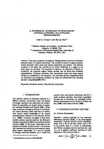
Definition 3 A straight line planar graph π is said to be a combinatorial pattern if π satisfies: (i) π is a 3-regular graph, (ii) π does not have a loop or multiple edges, (iii) the internal edges form a connected graph. If π1 and π2 are combinatorial patterns, then π1 and π2 are distinct if they are not isomorphic. The overview process for transforming a problem has been presented in our previous work 7 , and in brief is as follows. (i) Construct a condition to enumerate the number of vertices and edges by Euler’s formula and the condition of 3-regular graphs. (ii) Join the vertices with edges of every possible case that leads to a combinatorial pattern. (iii) Optimize each combinatorial pattern. Notation Let S be a unit square on the plane; π be a combinatorial pattern; and V , E and F be the set of vertices, edges and faces, respectively. Let V1 , V2 , V3 and V4 be the set of vertices on the top, left, bottom and right sides of the square, respectively; and similarly for Fi . Let V0 and F0 be the set of vertices and faces that are not adjacent to any side of the square. The cardinality of Vi and Fi are denoted by Vi and Fi . For faces in F1 , the faces are designated from the upper right corner proceeding anticlockwise by f11 , f12 , . . ., f1F1 . They are designated by starting at the upper left corner in the same manner by f21 , f22 , . . ., f2F1 . The third and fourth sides are designated similarly. We also obtain f1F1 = f21 , f2F2 = f31 , f3F2 = f41 , f4F4 = f11 . A face in the graph π is considered as a vertex in the dual graph π∗ . The notation f i j also represents a vertex in π∗ . If a face f i is adjacent to f j , we write f i ' f j , otherwise f i 6' f j . In the dual graph construction, if f i connects to f j , then f i ∼ f j , otherwise f i 6∼ f j . Fig. 1 illustrates the usage of provided notation. THE PROPOSED ALGORITHM Definition 4 Let π be a combinatorial pattern. The dual graph π∗ of π is called the dual combinatorial pattern. Triangulation process Suppose that π is a combinatorial pattern. Since π is a 3-regular graph, the dual graph π∗ of π is a planar graph composed of triangular faces. Hence we need to triangulate a set of vertices of a dual graph π∗ . Let Fout be a sequence of outer vertices, Fin be a set of interior vertices, F4 be a set of current www.scienceasia.org

Fig. 1 An example of a pattern π (left) and its dual graph π∗ (right). In this example, V1 = {v11 , v12 }, V2 = {v21 , v22 }, V3 = {v31 , v32 }, V4 = {v41 , v42 }, V0 = {v01 , . . ., v010 } and f11 ' f12 , f11 ' f42 , f11 ' f01 but f11 6' f02 . The numbers 1–4 in the left panel represent the side of the square.

triangles initially set to be empty, and P be a set of prohibiting connections. The following algorithm is a recursive process: (i) Join the vertices Fout sequentially. (ii) Triangulation Process: Consider Fin and Fout . A. If Fin 6= ∅, then 1. construct a triangle whose vertices are from two consecutive vertices ( fα fβ ) in a sequence Fout and a vertex fγ in Fin ; 2. add a triangle fα fβ fγ to F4 , delete fγ from Fin , and add edge fα fβ to P ; 3. insert fβ between fα and fβ in Fout ; 4. go back to (ii). B. If |Fout | ¾ 3, then 1. construct a triangle by three consecutive vertices fil , f jm , f kp in Fout that satisfy at least one of the following conditions: i 6= j or j 6= k or i 6= k; 2. add a triangle fil f jm f kp to F4 ; 3. delete f jm from Fout ; 4. go back to (ii). (iii) If |Fout | = 3 and Fin = ∅, then the process is complete. We note that the condition of P will be controlled in every step of the triangulation process. The prohibited condition will be provided in the next section. Fig. 2 illustrates the mentioned algorithm. The main process of this work is to generate all the possible dual combinatorial patterns. After all the dual combinatorial patterns are obtained, they are converted back to the respective combinatorial patterns and each pattern is optimized. To clarify, the overall process is summarized in the following

153

ScienceAsia 42 (2016)

We conclude that if T1 is symmetric with respect to T2 , the graphs generated from T1 will be isomorphic to those generated from T2 . Optimization process For each vertex (P, Q) in a combinatorial pattern, we denote the coordinates by P(x i , yi ) and Q(x j , y j ) and define q f (x i , yi , x j , y j ) = (x i − x j )2 + ( yi − y j )2 .

Fig. 2 Illustration of the triangulation algorithm: (a) Fin 6= ∅; (b) |Fout | ¾ 3.

steps. (i) Consider the number of faces on each side by doing an integer partition. To clarify this, we find the possible integer solutions of F0 + F1 + F2 + F3 + F4 = n + 4,

(2)

where the condition of F0 , . . ., F4 is determined in the next section. The solution of (2) is written as (F0 , F1 , F2 , F3 , F4 ). By fixing F0 , the following solutions are the same by rotating and flipping the square: (F0 , F1 , F2 , F3 , F4 ) = (F0 , F2 , F3 , F4 , F1 ) = (F0 , F3 , F4 , F1 , F2 ) = (F0 , F4 , F1 , F2 , F3 ), and (F0 , F1 , F2 , F3 , F4 ) = (F0 , F3 , F2 , F1 , F4 ) = (F0 , F2 , F1 , F4 , F3 ) = (F0 , F1 , F4 , F3 , F2 ). (ii) For each solution (F0 , F1 , F2 , F3 , F4 ) from (i), choose a representation of each face to be a vertex in the dual graph, and consider a set of Fout , Fin , F4 and Fproh . (iii) Triangulate a set Fin ∪ Fout by the stated algorithm. The results are called dual combinatorial patterns. Each prohibited connection will be denoted by an element { f ik , fjl } in P if f ik ∼ fjl is not allowed. (iv) Convert the dual combinatorial patterns to combinatorial patterns. (v) Optimize each combinatorial pattern. To speed up the generating process, and so avoid generating isomorphic patterns, the symmetrical patterns were considered as follows. Definition 5 Let T = (F0 , F1 , F2 , F3 , F4 ) be a solution of (2). T is symmetric with respect to X -axis if F1 = F3 . T is symmetric with respect to Y -axis if F2 = F4 . T is diagonal symmetric if F1 = F2 and F3 = F4 or F1 = F4 and F2 = F3 .

Then f is a convex function. When the domain of f is convex, minimizing f is of the type called convex programming. For each face in a combinatorial pattern, the maximum max f k (x i , yi , x j , y j ), π ∈ Π over all possible pairs of vertices is also convex. Hence the maximum (dmax ) of these max f k (x i , yi , x j , yi ) over all faces of π is convex. METHODS TO ELIMINATE THE UNNECESSARY PARTITIONS Although the proposed algorithm can generate all the possible combinatorial patterns, some of the generated patterns do not turn out to be the optimal partition. Those patterns are called unnecessary partitions. In this section, we provide the necessary conditions of a combinatorial pattern to be the optimal partition, which can help to eliminate the unnecessary combinatorial patterns. Note that the lemmas and theorems were constructed using the proved results of an earlier report by Guy and Selfridge 5 . Theorems to eliminate unnecessary partitions For a unit square S, we define A, B, C and D as vertices of the unit square, starting from the lower left corner and going anticlockwise. Hence A is at (0, 0). Lemma 1 (Ref. 7) A subdivided partition has a smaller or equal diameter than the original partition. By Lemma 1, dn is a non-increasing sequence. The following lemma and theorems show the necessary condition of being an optimal partition or combinatorial pattern. Lemma 2 For n ¾ 4, if the optimal partition has the combinatorial pattern π, then π has at least one vertex on each side. Proof : Suppose that there is a side which does not contain a vertex. Without loss of generality, assume that the side is AD. Since AD = 1, a piece containing AD has diameter of at least 1. However, p d4 = 2/2 < 1, a contradiction. 2 www.scienceasia.org

154

ScienceAsia 42 (2016)

D

C f11 x

f0i y

f31

A

B

Fig. 4 The initial combinatorial pattern of the solution (1, 3, 3, 3, 3) (left); the corresponding initial triangulating data (right).

Fig. 3 The situation f11 ' f0i ' f31 .

Theorem 2 For n ¾ 9, if the optimal partition has the combinatorial pattern π, then (i) π has at least two vertices on each side and (ii) π has at lease one interior piece. Proof : (i) The proof is similar to that in Lemma 2 but using d9 = 5/11. (ii) Suppose that π has no interior piece. Choose a point R( 12 , 12 ) in the square S. Hence there is a piece f i j . Since f i j is placed on the ith side, d(R, X ) ¾ 1/2 > d9 such that X is a point on the ith side that belongs to f i j . Thus π does not give the optimal diameter. 2

Theorem 3 (Ref. 7) For n ¾ 4, the combinatorial pattern π of an optimal partition may not satisfy either of the following conditions: (i) there is no edge from Vi to V j for i 6= j; (ii) there is no interior vertex incident to two vertices from opposite boundaries. We denote a set satisfying Theorem 3(i) by O , which we put in the set P . Theorem 4 For n ¾ 9, the combinatorial pattern π of an optimal partition may not satisfy the conditions: (i) there are two adjacent faces from opposite boundaries; (ii)there is no face adjacent to both f11 and f31 or both f21 and f41 .

Proof : (i) Without loss of generality, suppose that there is a face in F1 and a face in F3 that are adjacent. Denote a point on the first side which belongs to f1i and a point on the third side which belongs to f3 j as v1 and v2 , respectively. Hence there is x ∈ f1i ∩ f3 j such that d(v1 , x)+d(x, v2 ) ¾ 1. Hence the length of segment v1 x or x v2 should be greater or equal to 1/2 which means that d9 = 5/11 < 1/2. (ii) Suppose that f0i is a face satisfying f11 ' f0i ' f31 . Note that f11 and f31 are laid on the corners of a square which is shown in Fig. 3. The www.scienceasia.org

points A and C are on the boundary of the square which is the vertex ofpf31 and f11 , respectively. We note that d(A, C) = 2. By the assumption that f11 ' f01 ' f31 and the segment AC meets f11 , f01 and f31 , there are x ∈ f11 ∩ f01 and y ∈ f31 ∩pf01 such that d(C, x)+d(x, y)+d( y, A) > d(A, C) = 2. Hence one of the segments C x, x y, or yA has length p greater or equal to 2/3. This contradicts that p d9 = 5/11 < 2/3. 2 Hence we may define a partition or a combinatorial pattern to be unnecessary if it does not satisfy Lemma 2, Theorem 2, Theorem 3, or Theorem 4. COMBINATORIAL PATTERNS ENUMERATION To enumerate combinatorial patterns efficiently, we do not generate some of unnecessary patterns as they do not lead to optimal partitions. We put those unnecessary conditions in P . We enumerate patterns for n = 9 to 11 as follows. Enumeration of the case n = 9 Equation (2) is written in the form F0 + F1 + F2 + F3 + F4 = 13.

(3)

From Theorem 2, we have the conditions F0 ¾ 1 and F1 , F2 , F3 , F4 ¾ 3. Hence the only solution of (3) is (1, 3, 3, 3, 3). We consider the initial triangulation data in Fig. 4. From Theorem 4, we must avoid the situation f11 ∼ f01 ∼ f31 and f21 ∼ f01 ∼ f41 . Using a treediagram and the symmetry, the only condition we have is ( f01 6∼ f11 ) ∧ ( f01 6∼ f21 ). Since the solution (1, 3, 3, 3, 3) is symmetric with respect to the X -axis and Y -axis and is also diagonally symmetric, it suffices to consider the condition ( f01 6∼ f11 ) ∧ ( f01 6∼ f21 ) together with the condition from Theorem 3. Hence we have to

155

ScienceAsia 42 (2016)

Fig. 5 The initial combinatorial pattern of the solution (2, 3, 3, 3, 3) (left); the corresponding initial triangulating data (right).

triangulate: Fout = { f11 , f12 , f21 , f22 , f31 , f32 , f41 , f42 }, Fin = { f01 }, P = {{ f01 , f11 }, { f01 , f21 }} ∪ O . Enumeration of the case n = 10 Equation (2) is written in the form F0 + F1 + F2 + F3 + F4 = 14.

(4)

The lower bound condition is similar to the n = 9 case. The solutions of (4) are (1, 3, 3, 4, 3) and (2, 3, 3, 3, 3). Enumeration of (1, 3, 3, 4, 3) is similar to the case of (1, 3, 3, 3, 3) for n = 9 without the symmetry with respect to the Y -axis. We therefore consider the solution (2, 3, 3, 3, 3) by the initial triangulation data shown in Fig. 5. In this case, f01 was fixed with the conditions ( f01 6∼ f11 ) ∧ ( f01 6∼ f21 ), ( f01 6∼ f21 ) ∧ ( f01 6∼ f31 ), ( f01 6∼ f31 ) ∧ ( f01 6∼ f41 ) and ( f01 6∼ f11 ) ∧ ( f01 6∼ f41 ), followed by that for f02 in a similar manner. By the multiplication principle, this gives 16 conditions. Because (2, 3, 3, 3, 3) is symmetric with respect to the X -axis and Y -axis, and is diagonally symmetric, the condition is reduced to the following conditions: (i) ( f01 6∼ f11 ) ∧ ( f01 6∼ f21 ) and ( f02 6∼ f11 ) ∧ ( f02 6∼ f21 ), (ii) ( f01 6∼ f11 ) ∧ ( f01 6∼ f21 ) and ( f02 6∼ f11 ) ∧ ( f02 6∼ f41 ), (iii) ( f01 6∼ f11 )∧( f01 6∼ f21 ) and ( f02 6∼ f31 )∧( f02 6∼ f41 ). Thus we have to triangulate: Fout = { f11 , f12 , f21 , f22 , f31 , f32 , f41 , f42 }, Fin = { f01 , f02 }, and a set P will be considered by the above condition individually.

Fig. 6 Initial triangulating data for the solution (3, 3, 3, 3, 3) when n = 11.

Enumeration of the case n = 11 Equation (2) is rewritten as F0 + F1 + F2 + F3 + F4 = 15,

(5)

with the conditions F0 ¾ 1 and F1 , F2 , F3 , F4 ¾ 3. The solutions of (5) are (1, 3, 3, 3, 5), (1, 3, 3, 4, 4), (1, 3, 4, 3, 4), (2, 3, 3, 3, 4) and (3, 3, 3, 3, 3). The enumeration of the first four solutions are combinations of the case given above for n = 10 without any symmetric cases. Hence we specify the solution for (3, 3, 3, 3, 3). If F0 ¾ 3, the initial triangulating data will be larger. Hence we consider whether each corner is either a quadrilateral or an n-gon, where n ¾ 5. If a combinatorial pattern π consists of a quadrilateral at a corner, the dual combinatorial pattern π∗ consists of a triangle with the same corner. Along this part, we focus on the enumeration of the dual combinatorial pattern. The figures of dual combinatorial patterns are shown in Fig. 6 which indicates the initial triangulating data. The data in Fig. 6 are similar to the cases for n = 9 and 10 and were hence generated by considering the following cases. www.scienceasia.org

156 Case 1: every corner of the combinatorial pattern is a quadrilateral. For a quadrilateral Q at the corner of a combinatorial pattern π, there exists edges from two consecutive sides that are adjacent to v0k ∈ V0 for some k. Since v0k is a vertex of degree 3, there is an edge from v0k that is laid outside Q. Hence the f12 f22 , f22 f32 , f32 f42 and f12 f42 edges exist in the dual graph. The initial triangulation data is shown in Fig. 6 in case 1 with P = O . Case 2: only three corners of the combinatorial pattern are quadrilateral. In the dual graph, without loss of generality, suppose that f32 6∼ f42 . Thus a triangle f42 f32 f41 does not exist and an edge from f41 exists. If we consider the combinatorial pattern, the piece containing f41 is consecutive to the piece containing f32 . From theorems 2 and 4, there exists an internal piece consecutive to faces f41 and f32 . That is, there is f01 ∈ F0 such that f32 ∼ f01 ∼ f41 . The initial triangulation data is shown in case 2 of Fig. 6 with P = O . Case 3: only two consecutive corners of the combinatorial pattern are quadrilateral. Now, suppose that f32 6∼ f42 and f22 6∼ f32 . We can consider case 2 together with case 3 by supposing that two consecutive corners are quadrilateral. To avoid overlapping with case 1, we suppose that one corner is not quadrilateral and put no condition on the remaining corner. Without loss of generality, suppose that two upper corners are quadrilateral and the lower left corner is not a quadrilateral. The initial triangulation data is shown in the case 2+3 of Fig. 6 with P = O . Case 4: only two opposite corners of the combinatorial pattern are quadrilateral. Without loss of generality, suppose that the upper left and lower right corner are quadrilateral. Hence we have f12 ∼ f22 and f42 ∼ f32 . As with case 2, suppose that there is f01 ∈ F0 such that f31 ∼ f01 ∼ f32 . We can leave the condition of the upper right corner and employ the condition f12 6∼ f42 . Case 5: only one corner is quadrilateral in a combinatorial pattern. Suppose that there exists a triangle f32 f41 f42 in a dual combinatorial pattern. As with case 2, there exists f01 , f02 , f03 ∈ F0 such that f12 ∼ f01 ∼ f21 , f31 ∼ f02 ∼ f32 and f11 ∼ f03 ∼ f42 , which is shown in case 5 of Fig. 6. In the dual combinatorial pattern, however, we can combine cases 4 and 5 by determining one corner as a triangle, omitting the occurrence of triangle in the two opposite corners, and put no condition on the remaining corner. The initial triangulation data is shown in case 4+5 of Fig. 6 with P = {{ f02 , f11 }, { f03 , f31 }} ∪ O . www.scienceasia.org

ScienceAsia 42 (2016)

Case 6: every corner in a combinatorial pattern is not quadrilateral. Because we determined that each corner is not quadrilateral, there are edges from the corner point of the dual combinatorial pattern, i.e., face f11 , f21 , f31 , and f41 , as shown in case 6 of Fig. 6. Define points a, b, c and d as in Fig. 6 case 6. Since we have three interior points, there are two possible cases as follows. Subcase 6.1 a and b coincide, and c and d coincide. In subcase 6.1 of Fig. 6, we denote the merged point from a and b as f02 and the merged point from c and d as f01 . Let f03 be the remaining internal vertex. Hence we triangulate the data shown in subcase 6.1 of Fig. 6 with P = {{ f01 , f31 }, { f01 , f41 }, { f02 , f11 }, { f02 , f21 }}. Subcase 6.2: c and d coincide, but a and b do not coincide. Firstly, we show that the initial triangulation data in this case appears in the subcase 6.2 of Fig. 6, i.e., a ∼ f32 and b ∼ f32 . Denote a vertex f01 as with subcase 6.1 and let a and b be f02 and f03 , respectively. It suffices to construct a triangle f02 f31 f32 and f03 f32 f41 by the following arguments. Note that the edge f31 f32 must be contained in a triangle. From Theorem 4, f01 , f22 , f41 and f42 may not be the vertex of this triangle. To ovoid overlapping with the previous subcase, f02 must be the other vertex of that triangle. For a triangle with respect to f32 f41 , a similar argument was applied for the vertex f03 . Hence, in this case, we will triangulate with the initial triangulation data obtained in subcase 6.2 of Fig. 6 with P = {{ f01 , f31 }, { f01 , f41 }, { f02 , f11 }, { f03 , f21 }}. COMPUTATIONAL EXPERIMENTS We implemented the provided framework using MATHEMATICA 9.0 with NMinimize, an optimization tool for finding the global minimum of a function. We let dn denote the optimal diameter shown in the original results 5 , and Dn the optimal diameter obtained from our proposed algorithm. In the computations we used a default setting for which the working precision was equal to 16. Note that the optimization in this work is convex programming. In the case for n = 11, we can generate 4642 distinct combinatorial patterns that satisfy our conditions. Fig. 7 shows the optimized results from the combinatorial patterns for each n. From the experiments, d9 = 0.454545, D9 = 0.454545, d10 = 0.436467, D10 = 0.436467. In the case of D11 , the experimental result yields D11 = 0.416777 such that 0.388730 < D11 < 0.416778, which fits to the bound 5 . The results show that our results agree with their results in the cases of n = 9 and 10, and

ScienceAsia 42 (2016)

157 4. Graham RL (1967) On partitions of an equilateral triangle. Can J Math 19, 394–409. 5. Guy RK, Selfridge JL (1973) Optimal covering of the square. Coll Math Soc János Bolyai 10, 745–99. 6. Jepsen CH (1986) Coloring points in the unit square. Amer Math Mon 17, 231–7. 7. Chaidee S, Wichiramala W (2013) Numerical approach to the optimal partitioning of a square problem. In: Proceedings of the AMM, Krabi, pp 199–206.

Fig. 7 The combinatorial pattern (left) and the optimized results (right). Results of n = 9 (top), 10 (middle), 11 (bottom).

D11 in this study also agrees with the prediction of Guy and Selfridge 5 . Acknowledgements: The authors wish to thank the Development and Promotion of Science and Technology Talents Project by the Institute for the Promotion of Teaching Science and Technology, Ministry of Education, Thailand for the authors’ scholarship. We also would like to thank R. K. Guy for his suggestion and for providing material of his work, and C. Likitvivatanavong for valuable comments and suggestions. This study is partially supported by the 90th Anniversary of Chulalongkorn University Fund (Ratchadaphiseksomphot Endowment Fund). REFERENCES 1. Wenceslas GK, Lipman J (1958) Elementary problems and solutions: E1311. Amer Math Mon 65, 775. 2. Thompson GC, Munkres JR, Veech WA, Page Y, Goldstone LD (1959) Problems for solution: E1371-E1375. Amer Math Mon 66, 512–3. 3. Page Y, Selfridge JL (1960) Elementary problems and solutions: E1374. Amer Math Mon 67, 185. www.scienceasia.org