Prentice-Hall, USA. Gili Ripoll, J.A. (1988) Modelo microestructurado para medios granulares no saturados. PhD thesis,. Universidad Politecnica de Cataluña,.
A Numerical Implementation to Simulate Fluid-Mechanical Processes in Sand Production Using Discrete Elements R. Q. Velloso
Dept. of Civil Engineering, Catholic University, Rio de Janeiro, Brazil
E. A. Vargas Jr.
Dept. of Civil Engineering, Catholic University, Rio de Janeiro, Brazil
J. L. E. Campos
Dept. of Civil Engineering, Catholic University, Rio de Janeiro, Brazil
C. Gonçalves
Cenpes-Petrobras, Rio de Janeiro, Brazil
Abstract
The present work presents details of the numerical implementation of discrete elements under fluid flow, in order to analyze sand production processes in oil producing wells. Initially, a description of sand production processes is made. Subsequently, considerations are made regarding discrete elements and their application to the behaviour of granular materials. In particular, coupling schemes of discrete elements with one and two phase flow (oil-water) are presented. Finally, a few illustrative examples obtained with the implementations at present stage of the development are presented. 1 INTRODUCTION A number of problems in the oil industry are associated with sand production in oil producing wells equipment damage by abrasion, loss of production due to cleaning of separation chambers, difficulties in the treatment and discard of the produced sand and even safety problems in the platforms. Surface equipments can also be affected and the effects of sand production in the reservoir itself are yet not well understood. The practical solutions used presently for the remediation of the problem are (1) installation of gravel pack, in operations of elevated costs with impact in the well PI (productivity index) (reductions of PI in the order of 40 to 60 % registered at Campos basin) and (2) reduction in the well production (tests in the RJS-345 pointed at a 50 % reduction) in the production rates of the well.
In order to (1) establish appropriate solution measures and (2) investigate novel controlling techniques, it becomes necessary to develop laboratory and analytical/numerical procedures to simulate sand production processes under the operation conditions normally found during the life time of the producing wells. The paper presents developments associated with an ongoing project aiming at the understanding of sand production processes under the conditions normally found at Campos basin, the most important oil producing province in Brazil. The project involves both experimental and analytical/numerical activities. The present paper concentrates in the numerical activities. In particular, it will focus on applications of discrete elements to simulate sand production processes. Evidences from laboratory studies and field observations point to the fact that the sand production mechanisms
change considerably when two-phase flow is considered. During the life time of a well, especially during the later years of oil production, the so called water cut condition may happen. This condition is particularly relevant to wells in poorly consolidated or unconsolidated sandstones. The paper addresses this problem by presenting a formulation for the numerical simulation of sand production as a coupled hydromechanical process under two-phase flow using discrete elements. Preliminary results concerning a 2D numerical implementation of the proposed formulation are presented. 2 THE METHOD OF DISCRETE ELEMENTS AND ITS UTILIZATION TO SIMULATE SAND PRODUCTION PROCESSES In dicontinua such as fractured and granular media, forces are transferred through discrete units. In the case of fractured media, these units are blocks of rock and in granular media they are particles. It is usual in the engineering practice to simulate the mechanical behaviour of such media through the mechanics of continua. A realistic constitutive law for the representation of such media should provide an adequate description of effects such as anisotropy, stress path dependency, dilatancy and confining stresses dependency. Most of the constitutive models in existence does not contemplate in one or more aspects, in realistic fashion, the processes that occur due to the particulate, discrete nature of such media. Discrete elements are on the other hand, an alternative to the modelling of discontinua in relation to the usual methods utilized in the classical mechanics of continua. It has been used by now for more than thirty years in Geotechnical Engineering in the
modelling of fractured and granular media as early references suggest (Trollope, 1968 and Hayashi, 1966). In the seventies, a larger number of works appeared in particular the works by Cundall (Cundall, 1971 and Cundalll and Strack, 1979). Cundall presented examples of utilization of the DEM both for the simulation of both fractured media composed of rigid blocks and granular media formed by disks. An important contribution by Cundall was the introduction of the process of dynamic relaxation to solve the equilibrium equations for discrete media. Through dynamic relaxation, it becomes possible to solve complex problems involving physical and geometric non-linearities resulting from the interaction mechanisms between discrete units. Since the initial contributions, a number of applications of DEM were presented in Geotechnical Engineering, as for example in Rock Mechanics in the simulation of underground excavations (Lorig and Brady, 1984; Lemos, 1987), and in rock structure interaction (Ting and Corkum, 1988). Initially, DEM applications concerned dry media. Subsequently, extensions and adaptations were done to simulate rockfluid interaction problems in fractured media (Vargas Jr., 1982; Lemos, 1987; Kafritsas and Einstein, 1987 ; Harper and Last, 1989). In these simulations, the influence of water pressures generated by flow upon block equilibria was taken into account. Flow and equilibrium are in fact coupled processes and the numerical simulation should contemplate that fact. In the case of particulate media, more sophisticated implementations appeared ( Rothemburg and Bathurst, 1989) and more recently, attempts were made to simulate the hydromechanical coupling (one phase flow) in sand production situations in oil wells ( Thaliak and Gray,
1995; Dorfman et al, 1997; O´Connor et al, 1997; Preece et al, 1999; Cook et al, 2000). Two phase flow however has not yet been treated in a systematic way. Exception to that are the works of Gili (1988) and more recently of Gili and Alonso, (2002) where an application was presented for two-phase fluids (water-air) in order to simulated saturatedunsaturated flow in soils. It is not of the authors' knowledge applications to wateroil flow conditions. The present paper addresses this condition. Until recently, the DEM was basically for academic utilization. Nowadays however, its utilization to solve practical problems becomes more and more frequent.
where m is the mass of the element and Ii are the moments of inertia regarding the centroid of the element. (Fi)N and (Mi)N are the forces and moments respectively in the centroid of the elements resulting from the forces Fni and Fti acting at the contacts between the elements.
3 NUMERICAL IMPLEMENTATIONS OF DEM AND DATA STRUCTURES USED In this section, a brief exposition of the DEM is presented together with the implementations carried out. The numerical implementation used in the present paper uses dynamic relaxation, which consists in obtaining the solution of a static problem through its dynamic equations. This is achieved when the dynamic problem is correctly damped, avoiding oscillations.
Figure1 –Force and moments for two neighbouring particles Taking into consideration that the acceleration of a discrete element is constant during a time interval, the velocity of the element is given by:
(x i ) N + 1 = (x i ) N − 1 + 2
3.1
Formulation of DEM as applied to disks Figure 1 shows two interacting discrete elements (disks) representing granular materials. Newton's second law for each discrete element can be written as: m(x i )N = (Fi )N
( )N = (M i )N
I i θi
i = 1, 2, 3
(1)
2
(θi )N+ 1 = (θi )N− 1 + 2
(Fi )N ∆t m
(M i )N ∆t
(2)
Ii
2
and the space coordinates of the centroid and its rotation are given by :
(x i )N+1 = (x i )N + (x i )N+ 1 ∆t
(θi )N+1 = (θi )N + (
)
2
θi N+ 1 2
∆t
(3)
Based on the displacements and rotations of the elements, one is able to determine
the contact forces between elements. Contact forces are calculated from the increments of normal and tangential displacements (∆n, ∆s) existing at the contacts. These increments are obtained by using rigid body movements for each element together with linear and angular velocities at the element centroid in a discrete time interval : c ( ) 1 n i ∆t N + 2 2 1 (∆s )N+ = (x B − x A )N+ 1 t ic − 2 2 (θ A R A + θ B R B )N+ 1 ∆t
(∆n )N+ 1
= x Bi − x A i i
i
i
(4)
(M )
2
(Fn )N+1 = (Fn )N + k n (∆n )N+ 1 (Fs )N+1 = (Fs )N + k s (∆s )N+ 1
2
(5)
2
where kn and ks are the given normal and tangential stiffnesses at the contacts. The constitutive relationship at the contacts does not need to be linear. In principle tensile (opening) forces at the contact are not allowed. Contacts can therefore be broken at any time in the analysis and can eventually be recreated at a later times. Shear stresses and the possibility of slip between particles are controlled in a simple way by friction at the contact. Two particles will slide one in relation to the other when the tangential force at the contact exceeds a limiting value:
Fs ≤ Fsmax
(Fi )kN+1 =
i
and the contact force components are given by :
Fsmax = Fn tan φ
where Fs is the tangential force at the contact and φ is the friction angle. More sophisticated models can easily be implemented. After the determination of the forces at every contact, an update in forces and moments at the element centroid is made. This update is carried out by summing up all forces and moments at the contacts of one particle:
(6)
k N +1
nk
((F )
n =1
=R
k
c n N +1 n i
nk
+ (Fs )N +1 t ic
((Fs )N+1 )
)
(7)
n =1
where nk represents all contacts of an element `k´ and Rk is the element radius of element ´k´. Due to the dynamic nature of the algorithm, it is necessary to that both the damping (not shown in the above equations) and time interval be controlled in order to guarantee both convergence and stability. Figueiredo (1991) presents a synthesis of the methods of control of both processes (damping and time step) in order to control the algorithm appropriately. 3.2 Numerical Implementation Details Extensive use of Object Oriented Language (OOL) was used in the development of a library that implements the DEM. The use of OOL is particularly convenient when aspects such as maintenance and eventual extensions are considered. C++ programming language was used in the implementation of a library (DEMLib) which is responsible for the analysis of problems involving discrete elements. The library consists in a set of classes which define the basic objects that will be used in the implementation of the DEM.
The class cBlock represents a generic discrete element and contains data referring to physical and geometrical informations, the methods used in the calculations. From class cBlock, one defines other classes which are specializations for the geometric type of the element, a disk, a polygon or a sphere as depicted in Figure 2.
Figure 2 –Components of the class cBlock Other classes are defined with the objective of organizing the implementation of the method so make easier future extensions. cWall: Defines a boundary condition for the problem by specifying rigid walls, boundaries to which the elements will be in contact. The walls will be defined, in the 2D case as straight lines, polygonals or arcs. Figure 3 presents a hierarchy of classes that defines the types of walls available in the library.
Figure 3 –Components of the class cWall cLink: Defines the types of contacts that can be used in analysis. The contact types available in the library are relative to contacts between elements and between elements and the wall. Figure 4 presents a class hierarchy that defines the contact types that can be used during analysis.
Figure 4 –Components of the class cLink cBox : defines a class responsible for the definition of subdomains that will be used in the determination of contacts between elements and other elements and walls. For this class only two types are presently defined: 2D and 3D boxes. cDamping : Defines the damping types that can be used in the analysis. Figure 5 presents a class hierarchy used to define damping types.
Figure 5 Components of the class cDampingA graphical application was developed (program Sand) associated with DEMLib. It uses the available resources in the library to simulate a granular medium. This application was developed using programming languages C and C++, the Toolkit IUP/LED (Levy et al, 1996) and the graphical system CD (Tecgraf/PUC Rio, 1999). The program Sand (see Figure 6) offers the following facilities: • Graphic interface for visualization of the analyses steps • Interactive definition of the walls that define the boundary conditions and the disks that represent the granular medium
• •
Visualization of contact forces acting at the element centroid Interface with Lua (Figueiredo, et al, 1996) programming language allowing the generation of disks with specified dimensions according to rules defined by the user
25
2
0
3
2
6
1
0
9
2
4
12
24
3
7
11
3
1 15
22
1
5
8
10
4 13
5 16
6 18
7
21
14
17
19
20
23
2
0
6
1
9
0
3
0
7 15
11
14
8
16
8 14
5
7
13
5
13
6
3
4
12
1
12
2
10
4
18
9 17
21
10 19
11 20
Figure 7 – Particle structure and associated pore geometry Figure 6-Box filled with particles4 ONE AND TWO-PHASE FLOW IN DISCRETE PORES 4.1
Generation of pore network.
The first step in the flow evaluation in pores is the generation a pore network. It is built from the element information generated in program Sand. Program Sand generates a data structure for particles, walls and contacts as described in the previous sections. From the existing structure, an algorithm based in the work of Gili (1988) was created in order to generate the pore network (see Figure 7). One should notice that the contact between two particles represents, in the flow network, a conduct between two pores.
4.2
One-phase flow
The law of mass conservation for one phase transient flow in one pore (admitted incompressible at the present stage) can be written as:
i
−
∂ (ρv i ) ∂ρ = ∂x i ∂t
(8)
where ρ is the fluid density (ML-3) and v is the fluid velocity (LT-1). The left hand side of the equation refers to the summation of the mass rates of fluid entering or leaving the pore in regard to all pores connected to the analysed pore. The term on the right hand side is the mass time rate due to water expansion. This term is controlled by the fluid compressibility β (F-1L2): β=
1 ∂ρ ρ ∂p
(9)
where p is the fluid pressure (FL-2). Expanding the term on the lhs of expression (8) and knowing that ρ.∂vi/∂xi is much larger than the term vi.∂ ρ/∂xi. (Freeze & Cherry, 1979), introducing Darcy´s law and still substituting equation (9) in equation (8), one obtains:
i
∂ k ij ∂p ij ∂x i µ ∂x ij
=β
4.3 Two-phase flow The continuity equations, expressing mass conservation of both phases, one which is a wetting phase and a nonwetting phase (admitting an incompressible medium) are given by: − i
∂p j
(10)
∂t
i
where p is the fluid pressure, k is the conduct permeability and µ is the dynamic viscosity of the fluid (FL-2T). A finite difference scheme was used for the solution of (10). The scheme used was an explicit one. The reason to maintain an explicit algorithm was, besides maintaining a compatibility with the dynamic relaxation scheme of the particle code, to have a better control of possible changes of the pore network during the calculation cycles. The scheme makes it possible for pores to disappear or to be created along time. The fluid pressure is obtained according to the following equation: p nj +1
=
p nj
∆t + β
k ij i
∆x ij2 µ
(
p in
−
p nj
)
(11)
In the case of 2D analysis, it is admitted that the conduct between the two pores can be represented by a cylindrical pipe whose diameter is proportional to the area of the pores. It is therefore assumed that the conductivity of the conduct will be proportional to the pore areas that it connects. It is established through a Poiseuille type relationship.
−
∂ (ρ w v wi ) ∂ρ w ∂S w = Sw + ρw ∂x i ∂t ∂t
(12)
∂ (ρ n v ni ) ∂ρ ∂S = Sn n + ρ n n ∂x i ∂t ∂t
where the summation refers to the connected pores to the one being analysed, ρw and ρn are the densities , vw and vn are the velocities and Sw [-] e Sn [] are the saturations of the wetting and non wetting phases respectively . Following the same procedure already presented for one phase flow, substituting Darcy's law in equations (12) and introducing the compressibility for each phase (equation (9)), one obtains the following set of partial differential equations:
i
∂ k i k rwi ∂p wi ∂x i µ w ∂x i
Swβ w
i
∂p w ∂S w + ∂t ∂t
∂ k i k rni ∂p ni ∂x i µ n ∂x i
Sn β n
=
(13) =
∂p n ∂S n + ∂t ∂t
where k [L2] is the intrinsic permeability, krw [-] and krn [-] are the relative permeabilities, µw and µn are the dynamic viscosities, β w and β n are the compressibilities and pw and pn are the pressures of the wetting and non-wetting
phases respectively. These equations are coupled through the capillary pressure relation: Pc (S w ) = p n − p w
(14)
where Pc is the capillary pressure [FL-2], and are subjected to: (15)
Sn + Sw = 1
Equations (14) and (15) can be substituted in equations (13) so that they are expressed in terms of pn and Sn : ∂ k i k rwj ∂p ni ∂Pci ∂S ni − ∂x i µ w ∂x i ∂S n ∂x i
i
(1 − S n )β w i
Sn β n
(16)
=
∂p n ∂S n + ∂t ∂t
As with one phase flow, the numerical solution of equations (16) is obtained through an explicit finite difference scheme which can be written as:
i
n (Tnij (p ni − p nj )) i (Twij ((p ni − p nj ) − dPcnij (Sni − Snj ))) =
S njβ n 1 ∆t 1 − S nj β w
(
p nnj+1 S nnj+1
)
− p nnj − S nnj
1 − 1 − S nj β w dPcnj − 1
(
k rij k nij ∆x ij2 µ n
dPcnij =
,
Twij =
k rij k wij ∆x ij2 µ w
∆Pcij
(18)
∆S nij
For the determinations of permeabilities kwij, knij, and of dPcnij, an upstream weighing scheme was used (Aziz and Settari, 1979) defined for knij, for example as :
k nij =
k n (S ni ) , if flow is from i
( )
k n S nj
to j , if flow is from j to i
(19)
=
∂p ni ∂Pc ∂S ni ∂S − − n ∂x i ∂S n ∂x i ∂t
∂ k i k rni ∂p ni ∂x i µ n ∂x i
Tnij =
n
)
(17)
where the superscripts n and n+1 refer to the time step and :
4.4 Determination of the relationship Pc x Sw One important aspect in two phase flow is the relationship Pc x Sw. A simple model will be presented here to determine this relationship. It contains the following assumptions: • particles are spheres of radius R, equal and tangent in one point • The interface between the wetting and non-wetting phases is approximated by a toroid • the toroid is tangent to the particles (the contact angle interface –solid is zero) having an angle θ on the particles Figure 8 shows the simplified model of the meniscus. By knowing the form of the meniscus, it is possible to calculate the volume of the wetting fluid existing at the meniscus. By knowing the degree of saturation of the wetting fluid Sw in the pore, one is able to determine the wetting angle θ, by equating the volume of the
wetting fluid in the pore to the volume of the menisci existing in the pore. The capillary pressure at the interface , Pc, can be calculated through Laplace´s equation, which be expressed in a simplified way by : Pc =
2γ r2
(20)
where r2 is the radius of the interface (see Figure 8) and γ is the interfacial tension (FL-1). By using the relationship between r2 and the angle θ, and with the particle radius R in the above equation, one obtains: Pc (S w ) =
2γ cos θ R (1 − cos θ)
(21)
The angle θ is dependent on the degree of saturation of the wetting fluid Sw.
Figure 8 – Geometry of the meniscus
•
Transfer of seepage force and capillary pressures to the particles
The update of the pore network influences flow as it alters the geometric characteristics of the pores individually and of the pore network, allowing formation as well as disappearance of the pores. In the present implementation, no allowance was made for the rate of volume change of the pore space. It will however be taken into account in later stages of the work. The seepage forces together with the capillary forces influence in the particles movement. The seepage force is obtained by the integration of the fluid pressure along the area belonging to this pore (see Figure 9). In the case pf two-phase flow, the pore pressure is obtained in the following manner: p = S w .p w + S n .p n
(22)
Figure 9 – Determination of the seepage force, Fp The capillary force is obtained through: (23)
5 FLUID-MECHANICAL COUPLING
Fc = π(Rsinθ )2 Pc
The fluid mechanical coupling can be implemented by means of two processes: • the generation and updating the pore network due to the movement of particle
where θ is the wetting angle (see Figure 8), R is the particle radius and Pc is the capillary pressure. The capillary forces are attractive forces and they are oriented
along the lines that connect the centroids of neighboring particles. The coupling of the computer routines for the mechanical problem and the flow routines is done according the following steps: 1. A flow step is solved, obtaining pressures and pore saturations 2. Knowing pressures and saturations, one obtains seepage and capillary forces which are applied at the particles 3. The mechanical problem is solved in order to equilibrate the unbalanced forces 4. The pore network is updated returning to step 1. 6 ILLUSTRATIVE EXAMPLES A few illustrative examples concerning the formulations presented in the previous sections are presence in the sequence. 6.1
Construction of a model for sand production simulation studies This example demonstrates one way to generate a system of particles which will then be used in sand production studies. The example consists in the simulation of the settling of particles in order to fill a box. This box is limited by straight lines and an arc of circumference. In this cas, a line of particles (disks) with randomly generated particles is created. Under the action of gravity, the particcles move down onto the bottom of the box . As the particles contact the bottom of the box, another line of particles is generated and the process is repeated until the box fills up. The sequence of the simulation is shown in Figure 10.
Figure 10 –Sequences in the settling process of particles 6.2 Fluid-mechanic coupling The examples that follow demonstrate fluid-mechanical coupling for one and two-phase flow. The simulations were carried out for a geometry composed of twenty particles, each having a radius R=0.5 cm placed in a box of 12cm by 2 cm, as shown in Figure 11. The first example corresponds to a water flood situation. It consists of a medium initially saturated with oil (Sn =0.85) where water is injected at the left hand side end of the column in a way that the flow of oil is zero (qn=0), and the oil saturation at that end remains constant and equal to Sn = 0.10. The oil´s initial pressure along the column is 20 Mpa. These initial and boundary conditions are shown in Figure
11. Figure 12 shows the advance of the water saturation front.
0.06
qn = 0 Sn = 0.10
pn = 20MPa Sn = 0.85
pn = 20MPa Sn = 0.85
x-displacement [mm]
two-phase flow 0.05
one-phase flow
0.04 0.03 0.02 0.01 0.00
12cm
Figure 11 – Initial and boundary conditions in the two-phase flow simulation
0
2
4
6
8
10
time [s]
Figure 13 –Displacements of the crosshatched particle
7 CONCLUSIONS
Figure 12 – Advance of the water saturation front (t = 0s top, t = 5s middle, and t = 10s bottom) For the one-phase flow simulation, the same particle configuration used in the previous simulation was used. In order to compare the effects of the two types of flow (one and two-phase), the same values of water flow rate resulting from the conditions imposed in the two-phase simulation was imposed as boundary condition for the one phase flow simulation. This way, in both simulations the same water flow rate was used. Figure 13 shows the displacements of the crosshatched particle shown in Figure 11 for both one and two-phase flow. One is able to notice that the displacements for one phase flow are larger, possibly due to the effects of the capillary force.
The paper describes the present stage of development of a formulation for one and two-phase (water and oil) flow coupled with discrete particles. The aim of the implementation will be to simulate sand production studies in water flooding situations. The paper provides the details of the formulation and its numerical implementation.The results obtained so far, although limited, show promise in relation to the proposed objectives. REFERENCES Aziz, K & Settari, A. (1979) Petroleum Reservoir Simulation. Applied Science Pubs. Cook, B.K..; Noble, D.R.; Preece, D.S and Williams, J.R. (2000) Direct simulation of particle laden fluids. North American Rock Mechanics Symposium pp 279-286, Seattle. Cundall,P. and Stack,O.D. (1979) The distict element method as a tool for
research in granular media. Part 2. Technical report, Dept, of Civil and Mining Engineering, University of Minnesotta. Cundall, P. (1971) The measurement and analysis of accelerations in rock slopes. PhD thesis, University of London. Dorfmann, A.; Rothemburg,L.; Bruno, M.S, (1997). Micromechanical modelling of sand production and arching effects around a cavity. International Journal of Rock Mechanics & Mining Sciences, Vol. 34(3-4). Figueiredo, L.H.; Ierusalimsky, R. and celes, W. (1996) Lua: an extensible embedded language. Software: Practice & Experience., Vol. 26(6). Figueiredo, R.P. (1991) Aplicação da técnica de relaxação dinâmica à solução de problemas geotécnicos. MSc thesis. Dept. of Civil Engineering Catholic University, Rio de Janeiro. Freeze, R., and Cherry, J. (1979) Groundwater. Prentice-Hall, USA. Gili Ripoll, J.A. (1988) Modelo microestructurado para medios granulares no saturados. PhD thesis, Universidad Politecnica de Cataluña, barcelona, Spain. Gili, A., and Alonso, E., (2002) Microstructural deformation mechanisms of unsaturated granular soils. Int. J. Numer. Anal. Meth. Geomech., 26: 433-468. Harper, T.R. and Last, N. (1989) Interpretation by numerical modelling of changes of fracture system hydrayulics conductivity induced by fluid injection. Geotechnique, 3991). Hayashi, M. (1997). Mechanism of stress distribution in the fissured foundation. Proc. of the 1st Congress of the International Society of Rock Mechanics, Lisbon, Portugal
Kafritsas, J. and Einstein, H. (1987). Coupled flow-deformation analysis of a dam foundation with the distinct element method. 28th US Symposium of Rock Mechanics, pp 484-490, Tucson. Lemos, J. (1987) A distinct elemnt model for dynamic analysis of jointed rock with application to dam foundations and fault motion. PhD thesis, University of Minnesota. Levy, C.H.; Figueiredo, L.H.; Gattass, M.; Lucena, C. and Cowan, D. (1996) Iup/led: a portable user interface development tool. Software: Practice & Experience, Vol 26(7). Lorig,L.J. and Brady, B.H.G. (1984) A hybrid computational scheme for excavation in support design for jointed rock media. Design and Performance of Underground Excavation Conference, pp105-112, Cambridge, England. O´Connor, R.; Terczynsky,J.; Preece, D.; Klosek, J. and Williamns, J.(1997) Discrete element method of sand production. International Journal of Rock Mechanics and Mining Sciences, , 34(3-4). Preece, D.; Jensen, R.; Perkins, E. and Williamns, J. (1999) Sand production modeling using superquadric discrete elemnts and coupling of water flow and particle motion. 37th US Rock Mechanics Symposium, pp161-167, Vail Colorado. Rothemburg, L. and Bathurst, R.J. (1989) Analytical study of fractured anisotropy of idelaized granular materials. Geotechnique, 39(4).