Numerical Simulation: Field Scale Fluid Injection to a Porous Layer in relevance to CO2 Geological Storage Seunghee Kim*1, Seyyed A. Hosseini1, and Susan D. Hovorka1 1 Bureau of Economic Geology, Jackson School of Geosciences, University of Texas at Austin *Corresponding author: 10100 Burnet Rd, bldg.130, Austin, TX 78758, USA,
[email protected]
Abstract: CO2 geological storage can help to provide a “bridge” from a fossil-fuel dependent system to a more diversified energy portfolio. Pressure monitoring for an injection zone (IZ) and an above-zone monitoring interval (AZMI) has been under operation at a field-scale CO2 injection site, Cranfield, MS. Recorded pressure data in the AZMI revealed a certain amount of increase with no evidence of direct fluid flow between the IZ and the AZMI. We therefore attempted to interpret the field-measurement data from a geomechanical perspective. We conducted numerical simulations in which fully coupled calculation between fluid flow and geomechanics was implemented. Numericalsimulation results using COMSOL matched well with the field-measurement data obtained from the AZMI.
the vadose zones, have been utilized in monitoring migration of the CO2 plume at the Cranfield test site. In particular, pressure and temperature monitoring of an above-zone monitoring interval (AZMI) has been attempted for the first time in CO 2-injection history (Hovorka et al., 2013). Increase in fluid pore pressure was thought to be minimal if no massive communication were to occur between an injection zone (IZ) and an AZMI. However, measured increase in AZMI pore pressure at Cranfield was not small enough to be neglected, even though no evidence of CO2 leakage was found during the injection period (Meckel et al., 2013; Tao et al., 2012). Given this observation, we attempted to interpret measurement data from a geomechanical-response perspective.
2. Site Characteristics Keywords: CO2 geological storage, above-zone pressure monitoring, poroelasticity, COMSOL.
1. Introduction Burning of fossil fuels, and, thus, emission of carbon dioxide and other greenhouse gases to the atmosphere has been referred to as a main culprit in global warming. Coal and natural-gas power plants account for more than one-third of total carbon emissions worldwide (IPCC, 2005). However, fossil-fuel-based power plants should probably not be abandoned immediately, given our dependence on them for electricity. For this reason, Regional Carbon Sequestration Partnerships (RCSP), which consist of seven major regional partnerships in the United States, have been conducting a number of small- and large-scale CO2 injection projects to ensure the reliability of the carbon capture, utilization and storage (CCUS) and to raise it to an industrial scale (NETL, 2012). Cranfield pilot site, Mississippi, is one of the largest CO2 injection projects; as of July 2013, about 4 million metric tons of CO2 had been injected (Hovorka et al., 2013). Various monitoring strategies targeting different intervals, ranging from the injection to
The Cranfield site in southwestern Mississippi, USA, which comprises a nearcircular, four-way anticline, was active from discovery in 1943 to 1966 (Hosseini et al., 2012). During an idle period between 1966 and 2008, reservoir pressure recovered close to initial value via the incursion of formation water (Hovorka et al., 2013), and CO2 injection began in 2008 for enhanced oil recovery (EOR). The Tuscaloosa Formation overlies shale and sandstones of the Washita-Fredericksburg Formations in the Cranfield site (Figure 1). The injection interval is the lower Tuscaloosa Formation, fluvial conglomerates and sandstones (D/E sand), that are located at a depth of 3,167 m (10,420 ft); interval thickness ranges from 14 to 24 m. Porosity and permeability show wide variability (maximum porosity is ~0.32, and gas permeability is as high as hundreds of millidarcys; Ajo-Franklin et al., 2013). The main constituent is quartz (~80%), followed by chlorite (~12%; dominant coating and porefilling grains), iron-bearing dolomite, and calcite (Hosseini et al., 2012; Ajo-Franklin et al., 2013). Overlying the IZ is a sequence of mudstones and muddy sandstones that form the lower part of the
Cranfield confining system (Lu et al., 2011; Nicot et al., 2012). The upper Tuscaloosa Formation is a thin (10 to ~20 m), permeable interval that lies above the confining layers. This formation, ~3,060 m deep and located ~120 m above the injection interval, was chosen as the AZMI.
is 122~124°C; Hosseini et al., 2012). During CO2 injection, pressure and temperature had been monitored at the bottom holes of the injection well and the observation well, located 110m far from the injection well, for both IZ and AZMI. The increase in fluid pore pressure in the AZMI was recorded at ~∆P=40 kPa after ~7 months of CO2 injection operation.
Depth [m] -0
-300
-610
-910
-1220
-1520
-1830
-2130
-2440
-2750
-3050
-3350
Figure 1. Stratigraphic section for Cranfield test site (modified from Hovorka et al., 2011). The injection interval selected for the test was the lower Tuscaloosa Formation. The regional confining zone overlying the injection interval is middle Tuscaloosa “marine” mudstone and associated low-permeability facies. Upper Tuscaloosa formation was selected for the above-zone monitoring interval. Overburden includes diverse units and isolates the injection zone from shallow gas resources (Wilcox group) and underground sources of drinking water (USDW), which occur at depths of 30 to 600 m below land surface.
CO2 injection began in the study area on December 1, 2009. The initial injection rate, which was ~175 kg/min, doubled to ~330 kg/min on December 19, 2009. The injection rate was again increased to ~550 kg/min in May 2010. Injected CO2 is colder than hot formation water; the difference recorded at the bottom hole of the injection well is ∆T=~44°C (initial temperature
3. Use of COMSOL Multiphysics 3.1 Simulation Method We used the commercial software COMSOL to numerically experiment fluid injection into a porous-medium underground. The subsurfaceflow module in COMSOL contains predefined sets of equations adapted to many earth science applications (COMSOL, 2012). These equations include those for momentum transport (fluid flow), energy transport (heat transfer), and mass transport. The module also supplies predefined options for describing mass transfer by convection (advection), dispersion, diffusion, sorption, and reactions. In this module, a poroelasticity interface combines a transient formulation of Darcy’s law with a geomechanics interface. Of the two major constitutive equations defining poroelastic behavior, Darcy’s law describes the flow field in a poroelastic medium. The fluid equation comes from mass conservation:
( f ) ( f u) Q t
(1)
where ρf denotes density of fluid, φ porosity of the medium, and Q injection rate. Darcy’s velocity u and the storage model are:
k u (p f gh)
(2)
p ( f ) f S t t
(3)
where k is permeability of an injection interval, η is viscosity of fluid, and p and h are pressure and elevation head, respectively. Storage coefficient S is a function of Biot coefficient α, fluid bulkmodulus Kf, and drained bulk-modulus Kd:
S
Kf
( )
1 Kd
(4)
The other constitutive equation relates stress σ, strain ε, and fluid pore pressure p:
C p I
(5) Elasticity matrix C in Equation 5 must be measured under a drained condition. I denotes identity matrix. If Equation 5 is divided into volumetric and deviatoric parts, the deviatoric part (shear stress) is independent of porepressure coupling. Coupling in the volumetric part can be written as:
kk 3
K d vol p
(6)
where σkk denotes mean stress and εvol represents volumetric strain. The governing equations are fully coupled during numerical simulation, and computation iterates between these equations for each time step within a finite-difference method.
Table 1: Input parameters for numerical simulations
Parameters Young’s modulus Poisson’s ratio Drained bulk density Porosity Biot coefficient Permeability Bulk modulus of fluid Density of fluid Viscosity of fluid Injection rate
Value IZ & Else AZMI 17.5GPa 30GPa 0.15 0.3 2650kg/m3
2000kg/m3
0.25 1 64md
0.1 1 1nd 2.2GPa
1000kg/m3 0.001Pa·s 175→330→500kg/min
3.2 Model and Boundary Conditions Axisymmetric
We built the simulation model as simple as possible without losing geometric relevance to a field condition. The model retains an axisymmetric configuration in which the left side is a central axis (Figure 2). The AZMI is 120 m above the IZ, and these two intervals are the only layers with a high permeability value in the model. Other layers are assigned a low permeability value, k=1 nd (Table 1), so that the confining layer between the two permeable intervals acts as a hydraulic barrier. Thickness of the two intervals is identical, at 20 m. The right side of these two intervals is set at the fluid outlet. The top and bottom are set at the closed fluid boundary. In mechanical boundary conditions, a roller is imposed on the left and right sides and the bottom (i.e., perpendicular displacement is not allowed, whereas transitional displacement is allowed). The top surface is free to move. Radial and vertical boundaries are 10 km away from the left and 6 km away from the top, respectively, to avoid any boundary effect. A dot in the AZMI represents the location of monitoring point. Fluid injection, that is imposed on the left-end of the injection zone, is initially 175kg/min (0.1MtCO2/yr) and doubles after 19days, and increases again to 500kg/min (0.3MtCO2/yr) after 183 days. Total simulation time is about 230 days (≈107.3 seconds).
Surface
Location of field measurement
3,050m
110m Above Zone (AZMI) Fluid
Confining layer Injection Zone
20m 120m 20m
6km
10km
Figure 2. Simulation model and geometric conditions for numerical-experiments using COMSOL.
4. Result Numerical simulation yields an ideal response to bottom-hole pressure increase near the injection well: bottom-hole pressure exhibits a sudden increase corresponding to the onset of injection and/or change in injection rate (Figure 3). However, this typical response is not observed in the field data (Figure 4). Pressure monitoring actually suggests that bottom-hole pressure spiked during early initial injection then decreased to some extent to level off at ∆P~6.21 MPa until an increase in injection rate from 175 to 330 kg/min (Figure 4). This behavior implies that the IZ may have experienced some reactivation of existing discontinuities or hydraulic fracturing near the injection well. The likelihood of these geomechanical failures is able
31300
Pressure [kPa]
to explain the absence of another jump in bottom-hole pressure in the field data at ~180 days passed once injection began (Figures 4), as was suggested by Hosseini et al. (2012). Possible events of geomechanical failure might also explain the final increase in bottom-hole pressure being higher in the numerical-simulation results (∆P~14 vs. ∆P~9 MPa; Figure 4).
31250
Field data 31200
31150
Numerical simulation
31100
Injection rate [kg/min]
15
500
12
400 9 300
Injection rate 6
200 3
100 0
0 0
50
100
150
200
Increase in pressure ∆P [MPa]
-50
Bottom-hole pressure
600
250
0
50
100
150
200
250
Time [day]
Figure 5. Comparison of bottom-hole pressure between field-measurement data (dots) and numerical simulation results (solid line) for AZMI.
We were also able to investigate probable displacements at the surface: maximum value reached ~1.2mm at the central point after 230days (Figure 6).
Figure 3. Numerical simulation results: Imposed injection rate (dotted line) and resulting bottom-hole pressure near the injection well (solid line).
Pressure [MPa]
46
Numerical simulation
42
38
Field data
Vertical displacement [mm]
Time [day] 1.2 1 0.8 0.6
0.4 0.2 0 0
2
4
6
8
10
Radial distance [km]
34
30 -50
0
50
100
150
200
250
Time [day]
Figure 4. Injection-zone analysis: Comparison of bottom-hole pressure near injection well between field-measurement data and numerical simulation results.
When it comes to pressure increase in AZMI, field-measurement data and numericalsimulation results are in accordance, even if not totally consistent (Figure 5). Both graphs show in detail a jump immediately following CO 2 injection began (around zero time elapse) and exhibit another jump following increase in injection rate (~20 day time elapse). After the second jump, both graphs show relatively constant pressure. Absolute pore-pressure increase after ~230 days is also comparable (∆P~40 kPa for both graphs).
Figure 6. Distribution of vertical displacement at the surface, as a result of CO2 injection.
Finally, coupling of pore pressure-stress was observed during the numerical simulations (Figure 7). Specifically, increase in pore pressure is linked to increase in total stress (also decrease in pore pressure is linked to decrease in total stress). This coupling is more pronounced for total horizontal stress because lateral deformation is isolated within sedimentary basins. A summary of reported field data from many oil-production sites suggests that this porepressure–total-horizontal-stress coupling ratio ranges to 0.46