A one-dimensional model of cell diffusion and aggregation, incorporating volume filling and cell-to-cell adhesion K. Anguige∗, RICAM, Austrian Academy of Sciences, Altenbergerstr. 69, A-4040 Linz, Austria C. Schmeiser, Faculty of Mathematics, University of Vienna, Nordbergstr. 15, 1090 Vienna, Austria June 15th, 2007
Abstract We develop and analyse a discrete model of cell motility in one dimension which incorporates the effects of volume filling and cell-to-cell adhesion. The formal continuum limit of the model is a nonlinear diffusion equation with a diffusivity which can become negative if the adhesion coefficient is sufficiently large. This appears to be related to the presence of spatial oscillations and the development of plateaus (pattern formation) in numerical solutions of the discrete model. A combination of stability analysis of the discrete equations and steady-state analysis of the limiting PDE (and a higher-order correction thereof) can be used to shed light on these and other qualitative predictions of the model.
Key words or phrases: Cell-to-cell adhesion - Continuous and discrete models of cell motility Nonlinear diffusion equations - Ill-posed problems - Modified equations.
1
Introduction
There is by now a vast literature devoted to modelling the motion of cell populations in numerous biological contexts, such as bacterial aggregation and biofilm development, tumour invasion and the ensuing immune response, to name but a few. Of course, the mathematical nature of the resulting models depends very much on the situation under consideration, whereby it should be noted that in many contexts several modelling approaches, discrete and continuum, are possible. One problem in this area which has attracted a good deal of attention recently, and which will be the focus of this paper, is that of modelling aggregation in an initially dispersed population of cells which can interact via cell-to-cell adhesion; the motivation, here and in the literature, is to gain a better understanding of structure formation in developmental processes such as gastrulation and vasculogenesis in the early embryo, for example. In this connection, a number of authors have successfully used computational modelling to reproduce experimentally-observed aggregation patterns in single cell-type populations, as well as cell-sorting behaviour in mixed populations (see, e.g., ∗ e-mail:
[email protected]
1
[1, 3] and references therein). Almost without exception, the models employed have been of the discrete variety, reflecting the difficulty of writing down appropriate continuous models. A continuous, non-local model of cell-to-cell adhesion has recently appeared in the literature [1], although it should be remarked that this model does, nevertheless, contain a fixed small parameter (a measure of cell size), which is a characteristic feature of the corresponding discrete models. We note that continuum models are generally regarded as being more desirable than their discrete counterparts, insofar as they are expected to be more amenable to mathematical analysis, and therefore lead to greater physical insights, particularly when one is dealing with large numbers of particles. In a number of biological contexts where the cells under consideration are not very tightly packed (such as in the case of flagellar bacterial motion, for example), it is assumed that, on the macroscopic scale, cell motion is governed by a Fickian diffusion equation, possibly with the addition of chemotactic terms, reflecting the response to extracellular chemical gradients [4]. In this paper we make an attempt to generalise this type of model in a particular direction, such that consideration is given to an inhomogeneous distribution of particles which can to some extent move randomly, but whose movements are restricted by the effects of volume filling and, crucially, cell-to-cell adhesion. Under these conditions, we cannot, a priori, expect the cell motion to be governed by simple Laplacian diffusion. When deriving diffusive models for cell or particle movement from first principles, a popular method [5, 6] is to undertake a spatial discretisation of the biological domain, and to write down a master equation for a continuous-time, discrete-space random walk on the resulting lattice. More precisely, focusing attention on a uniform one-dimensional lattice, one defines ρi (t) to be the probability of a walker being at the point labelled by i ∈ Z, conditioned on being at i = 0 at t = 0, and assumes that this quantity evolves according to ∂ρi + − = Ti−1 ρi−1 + Ti+1 ρi+1 − (Ti+ + Ti− )ρi , (1) ∂t where Ti± (·) are the transitional probabilities per unit time of a one-step jump from i to i ± 1. Upon taking the continuum limit of (1), one ends up with a diffusion equation for the macroscopic density ρ(x, t), which might be, say, the classical Keller-Segel chemotaxis equation, or some variant thereof [4, 6, 7]. This is the approach that we shall adopt in this paper, our aim being to write down a conservation equation for a continuous distribution of adhesive particles on a bounded interval on the real line, whereby, as is standard, we wish to reinterpret the discrete quantity ρi as an approximation to the cell density ρ(x, t) at position x = xi := ih, rather than as a probability density. The discrete model investigated here has the (dimensionless) form Ti+ = (1 − ρi+1 )(1 − αρi−1 )/h2 ,
(2)
where the first factor models volume filling with a scaled maximal density 1, and the second is a simple model for adhesion, which assumes that the probability of a given particle jumping to the right is reduced by the presence of neighbours to the left; the definition of Ti− is analogous. Our results show that the value of the adhesion coefficient α ∈ [0, 1] determines the qualitative behaviour of solutions to this model; there is a critical value of α (= 34 ), below which initial inhomogeneities in the density profile simply diffuse away, resulting in a uniform density distribution at steady state, and above which pattern formation becomes possible. Our understanding of this qualitative dependence on α is aided by taking the continuum limit of the discrete model, and, indeed, an examination of the (rather thorny) relationship between the discrete and continuous models constitutes the heart of the paper; the limiting PDE for the density ρ turns out to be a nonlinear diffusion equation, with a ρ-dependent diffusivity which can become
2
negative for a range of values of ρ iff α > 34 . The fact that we are therefore dealing with an equation of backwards-heat type explains, in some sense, the instability giving rise to pattern formation in this high-adhesion regime. In cases where pattern formation occurs, the pattern emerges on rather a short timescale, and subsequently evolves into a two-valued, multi-peak plateau solution which remains stable over a very long period. For given initial data, the number of peaks in the pattern increases linearly with the number of mesh points, and this behaviour can be understood by carrying out a linear stability analysis of the discrete model. One can also extend the analysis of this (spatially) fast-oscillating behaviour as the mesh size h → 0, in a nonlinear fashion, by obtaining periodic steady-state solutions of a higher-order correction to the leading-order continuum equation with a blown-up spatial scale. The observed multiple-peak solutions of the discrete model, which are shown to be close to square-wave weak solutions of the limiting PDE, and which appear at first glance to be steadystate solutions, are in fact merely metastable, such that a coarsening process, involving merging of neighbouring peaks, is seen numerically over very long timescales, eventually leading to a steadystate solution with just a single peak (or trough). This is redolent of the behaviour observed in, for example, the Cahn-Hilliard equation for phase separation in alloys [8], and in certain models of chemotaxis with volume-filling [6, 7, 2]. In fact, when one comes to consider higher-order corrections of the full time-dependent continuum model, one is able to write down a fourth-order diffusion equation which is very much like the viscous Cahn-Hilliard equation, with O(h2 ) viscosity. The presence of the viscosity term entails that this corrected equation has a well-posed initial-value problem, as we are able to prove rigorously. The paper is organised as follows. In Section 2 the discrete ODE model is derived, and some elementary properties listed. In Section 3 we obtain the continuum limit of the model, whereby the qualitative difference between the low- and high-adhesion regimes becomes apparent; an analytical result on the long-time behaviour of solutions is stated for α < 43 . Section 4 contains our first batch of simulations of the discrete model equations. In Section 5 we carry out the linear stability analysis for the discrete model. In Section 6 we obtain weak steady-state plateau solutions of the continuum model, and finally, in Section 7, we investigate higher-order modifications to the continuum equation, obtaining approximate pleateau solutions thereof, stating our well-posedness result, and discussing the issue of metastability and coarsening with the aid of further simulations.
2
The Discrete Model
We consider a discrete distribution of particles on the interval [0, 1]. This interval is divided into N subintervals of length h, with endpoints xi = ih, i = 0, 1, ..., N ; the particle density at the lattice point xi is denoted by ρi , and we require 0 ≤ ρi ≤ 1. There is just one parameter in the model, namely the adhesion coefficient α ∈ [0, 1]; if α = 0 there is no cell-to-cell adhesion, and if α = 1 there is total adhesion. The model presented in the introduction leads, for i = 2, . . . , N − 2, to a net flux of particles from xi to xi+1 of the form Ji+1/2 =
1 [ρi (1 − ρi+1 )(1 − αρi−1 ) − ρi+1 (1 − ρi )(1 − αρi+2 )] , h
(3)
and the conservation equation for ρi is therefore Ji−1/2 − Ji+1/2 ∂ρi = , ∂t h for i = 2, . . . , N − 2.
3
(4)
In order to obtain boundary equations, we define J−1/2 = 0,
J1/2 =
1 [ρ0 (1 − ρ1 )(1 − αρ0 ) − ρ1 (1 − ρ0 )(1 − αρ2 )] , h
(5)
and JN +1/2 = 0,
JN −1/2 =
1 [ρN −1 (1 − ρN )(1 − αρN −2 ) − ρN (1 − ρN −1 )(1 − αρN )] , h
(6)
and demand that (4) also hold for i = 0, 1, N − 1 and N . Note that the truncated expressions for J1/2 and JN −1/2 are obtained simply by substituting i with 0 and N − 1, respectively, in the general expression (3), and then replacing the virtual quantities ρ−1 and ρN +1 with ρ0 and ρN , respectively. These choices ensure that the Neumann boundary condition at x = 0, 1 falls out in the continuum limit h → 0 (see Section 3). Our discrete model equations constitute a system of N + 1 ODEs for the ρi , and it is straightforward to prove the following. Theorem 1 The system (4), for i = 0, . . . , N possesses the following three properties. 1. Mass is conserved, i.e.
PN i=0
ρi (t) =
PN i=0
ρi (0) := M, ∀t.
2. The solution ρi (t) can never pass through 0 or 1, leading to the observation that if 0 ≤ ρi (0) ≤ 1 ∀i (as we demand) then we have the a priori bound 0 ≤ ρi (t) ≤ 1, and the result that the solution ρi (t) exists for all time, by standard ODE theory [9]. 3. One always has the uniform steady-state solution ρi = constant = solutions being examined in Section 5).
M N +1
(the stability of such
Finally, we note that, although plateau steady-state solutions taking the values ρi = 0, 1 can be constructed when α = 1, in general we have been unable to find non-uniform steady-state solutions analytically. Such solutions can, however, be found numerically for sufficiently large α; numerical solutions of the model are presented in Section 4, after an analytical interlude.
3
The Continuum Limit
Before presenting our numerical simulations of the discrete adhesion-diffusion model, it is, as we will see, instructive first to write down the continuum limit of the model as h → 0. To this end, it is convenient to note that the flux can be written as a finite difference, namely Ji+1/2 =
Ri − Ri+1 h
, with
¡ ¢ Ri = ρi 1 − α + α(ρi+1 − 1)(ρi−1 − 1) ,
(7)
and hence that the formal passage to the limit h → 0 in (4) gives the nonlinear evolution equation µ ¶ ∂ 2 K(ρ) ∂ ∂ρ ∂ρ = = D(ρ) , (8) ∂t ∂x2 ∂x ∂x where K(ρ) = ρ(1 − 2αρ + αρ2 ), the diffusivity is given by µ ¶2 2 4 D(ρ) = K (ρ) = 3α ρ − + 1 − α, 3 3 0
4
(9)
∂ρ and the boundary conditions are just ∂x = 0 at x = 0, 1. We immediately see by inspecting (9) that the mathematical character of (8) depends on the magnitude of the adhesion coefficient α, and we distinguish here between two possible cases.
Case (i) : 0 ≤ α
34 , to which we now turn our attention. Further analysis of the continuum model, and of the discrete model, will be carried out below.
4 4.1
Numerical Solutions of the Discrete Model The Numerical Algorithm
In order to solve the discrete model equations, we first rewrite (4) as
5
∂ρi 1 + 2 (ρi f (ρi−2 , ρi−1 , ρi+1 , ρi+2 ) − g(ρi−2 , ρi−1 , ρi+1 , ρi+2 )) = 0, ∂t h
(12)
where f (ρi−2 , ρi−1 , ρi+1 , ρi+2 ) =
[(1 − ρi+1 )(1 − αρi−1 ) + ρi+1 (1 − αρi+2 ) +ρi−1 (1 − αρi−2 ) + (1 − ρi−1 )(1 − αρi+1 )],
(13)
and g(ρi−2 , ρi−1 , ρi+1 , ρi+2 ) = ρi+1 (1 − αρi+2 ) + ρi−1 (1 − αρi−2 ). Next, we carry out a semi-implicit time discretisation, such that the solution, step (of size ∆t) is updated according to
(14) ρni ,
at the nth time
− ρni 1 ρn+1 i + 2 (ρn+1 f (ρni−2 , ρni−1 , ρni+1 , ρni+2 ) − g(ρni−2 , ρni−1 , ρni+1 , ρni+2 )) = 0, ∆t h i which can be rewritten as the explicit scheme ρn+1 = i
h2 ρni + ∆tg(ρni−2 , ρni−1 , ρni+1 , ρni+2 ) . h2 + ∆tf (ρni−2 , ρni−1 , ρni+1 , ρni+2 )
(15)
(16)
The boundary equations are handled similarly. Note that the algorithm (16) is unconditionally stable, in the sense that if 0 ≤ ρni ≤ 1 then clearly, from (13)-(14), 0 ≤ g(ρni−2 , ρni−1 , ρni+1 , ρni+2 ) ≤ f (ρni−2 , ρni−1 , ρni+1 , ρni+2 ), and hence 0 ≤ ρn+1 ≤ 1. i This algorithm, along with the corresponding boundary equations, can readily be implemented in Matlab, for example, and we now present some results of our simulations in the low- and highadhesion regimes, respectively.
4.2
Numerical Results for α
3 4
If we let α > 34 , and simulate the discrete model with initial data ρi (0) uniformly outside Iα , then the qualitative behaviour of solutions is just as described for α < 34 . If, instead, we simulate the model with α > 34 and ρi (0) ∈ Iα for some values of i, then something more interesting happens, as we expect from the analysis of Section 3. In Figure 2 we take the same data and the same mesh size as in Figure 1, but now we assume α = 0.95. The interval Iα , where D(ρ) < 0, is marked (here and henceforth) with dotted lines, clearly showing that the initial density hits this unstable region for some values of xi . 6
The evolution is very different from that observed with α = 0.1; one sees aggregation of particles around the largest peak, while elsewhere the inhomogeneities diffuse away. The bump to the right of the main peak depicted in Figure 2(d) settles down completely as t → ∞, leaving an essentially two-valued plateau solution at steady state. Note that, as far as we can tell, the plateau does not approach the boundary; it stays where it is. In Figure 3 we again take α = 0.95 and N = 100, this time displaying the evolution of broad, bell-shaped initial data, given explicitly by 2
ρi (0) = 2e−(1/(1−(2xi −1)
))
.
In Figures 3(c) and 3(d) we see the development of a pattern of aggregation, which subsequently remains stable over a timescale which is much (100-1000 times) longer than that over which the oscillations are initially set up - we return later on to the question of whether the multi-peaked solutions are in fact literal steady states. How can we explain the difference between the plateau-formation observed in Figure 2 and the oscillations seen in Figure 3 ? A clue to answering this question is provided by doubling the number of mesh points. In Figure 4 we take the same initial data as in Figure 2, but now we simulate the discrete model with N = 200, rather than N = 100 spatial points. As we see, the density profile evolves rather differently than in Figure 2; the largest peak builds up as before, but now develops an oscillation, while the second-largest peak, instead of diffusing away, forms an additional plateau. In those regions where ρi lies below Iα the solution simply flattens out again; the resulting two-valued, three-peak plateau solution remains stable on a very long timescale. Carrying out the same procedure with the initial data as in Figure 3, we obtain the simulation shown in Figure 5. As in Figure 3, we see oscillations develop, but this time the resulting pattern has twice as many peaks. In fact, one can continue doubling the number of spatial points, with the result that the number of peaks also continues to double, whereby, however, the simulations quickly become very messy (data not shown). These numerical results led us to wonder whether the linearisation of (4) about the uniform steady state might, for sufficiently large α, have unstable periodic eigenvectors, with the dominant mode having period (i.e. number of mesh points in one cycle) independent of the total number of mesh points N + 1. This turns out to be correct, as we show in the next section. Moreover, an analysis of weak steady-state solutions of the continuum equation (8) gives information on when we can expect to see plateau solutions at large times, and what the plateau values of ρi will be (see Section 6).
5
Linear Stability Analysis
The linearisation of (4) about the uniform state ρi = ρ takes the form ∂ρi 1 + 2 Ai j ρj = 0, ∂t h where the stability matrix A is given by A = D(ρ)A1 + αρ(1 − ρ)A2 ,
7
(17)
(18)
and the symmetric matrices A1 and A2 are 1 −1 −1 2 0 −1 0 0 A1 = 0 0 . . .. .. 0 0
A2
=
defined by 0
0
0
0
−1
0
0
0
2
−1
0
0
−1
2
−1
0
0 .. .
−1 .. .
2 .. .
−1 .. .
... .. . .. . .. . .. . .. .
..
..
.
.
0
0
0
0
0 0
−1 0
2 −1
2
−3
1
0
0
0
−3
6
−4
1
0
0
1
−4
6
−4
1
0
0 .. .
1 ..
−4 .. .
6 .. .
−4 .. .
0 0 0
0 0 0
0 0 0
1 0 0
−4 1 0
1 .. . 6 −4 1
... .. . .. . .. . .. . −4 6 −3
.
0
0 0 0 , 0 0 −1 1 0
(19)
0 0 0 . 0 1 −3 2
(20)
Theorem 3 The eigenvalues of A1 and A2 lie in the intervals [0, 4) and [0, 16), respectively. Moreover, A1 and A2 have identical eigenvectors, such that the zero eigenvalue of each has a 1-d eigenspace P spanned by the eigenvector ρi = const., and all other eigenvalues have eigenvectors satisfying ρi = 0. Proof. We first consider A1 , for which the general row of the eigenvalue problem, with eigenvalue λ and eigenvector ρj , is
Substituting the ansatz ρj = e
ijθ
−ρj−1 + (2 − λ)ρj − ρj+1 = 0. √ (where i = −1) into (21) leads to the auxiliary relation λ = 2(1 − cos θ).
(21)
(22)
If we can now find N + 1 values of θ such that the boundary conditions are satisfied then we will have the required N + 1 eigenvectors, with corresponding eigenvalues λ automatically in [0, 4). Suppose first that the matrix dimension N + 1 is odd, and, for convenience, let j = 0 index the middle row of the matrix. The boundary equations are then ρ− N −1 2
ρ N +1 2
= ρ− N , 2
= ρN . 2
8
(23)
Trying an eigenvector of the form ρj = cos jθ ensures that the two boundary equations (23) are equivalent, and thus we merely require cos ( N2 + 1)θ = cos N2 θ. Using elementary trigonometrical N formulae, we see that this condition is satisfied by taking θ = θk := N2kπ +1 , k = 0, . . . , 2 , giving N us 2 + 1 eigenvectors with distinct eigenvalues λ ∈ [0, 4). In a similar way, one sees that the remaining N2 distinct eigenvalues can be obtained by taking the eigenvector to be ρj = sin jθk , with N θk = (2k+1)π N +1 , k = 0, . . . , 2 − 1. From our explicit formulae, it is clear that the zero eigenvalue of A1 has a 1-d eigenspace spanned by the eigenvector ρi = const.. We note that the case N + 1 even is handled similarly, and that the expression for the eigenvalues is exactly the same as for N + 1 odd. Turning to the matrix A2 , and once more assuming that N + 1 is odd, we see that the general row of the eigenvalue equation is ρj−2 − 4ρj−1 + (6 − λ)ρj − 4ρj+1 + ρj+2 = 0,
(24)
such that j = 0 indexes the centre of the matrix. We again try the ansatz ρj = eijθ , this time obtaining the auxiliary relation λ = 4(cos θ − 1)2 ,
(25)
and we look for choices of θ which satisfy the boundary conditions. Generally, there is a pair of boundary equations coming from the first two eigenvalue equations, and another pair coming from the last two. However, taking ρj = sin jθ implies that these pairs are equivalent, and it is therefore enough to consider the last pair, which can be written as ρ N +1 − ρ N
= 0,
(26)
−ρ N −1 + 4ρ N − 4ρ N +1 + ρ N +2
= 0.
(27)
2
2
2
2
2
2
Now, given our ansatz for ρj , (26) holds iff cos
(N + 1)θ θ sin = 0, 2 2
(28)
and (27) holds iff µ ¶ θ (N + 1)θ θ 1 + 4 sin2 cos sin = 0. 2 2 2
(29)
N N Taking θ = (2k+1)π N +1 , k = 0, . . . , 2 − 1 satisfies these boundary conditions, and gives us 2 distinct eigenvalues ∈ (0, 16). A similar calculation shows that the remaining eigenvectors and eigenvalues N (including the zero eigenvalue) are obtained by taking ρj = cos jθ, with θ = N2kπ +1 , k = 0, . . . , 2 . The case N + 1 even is treated analogously; the expression for the eigenvalues is identical to the case N + 1 odd, and the eigenvectors P are again the same as those of A1 . Finally, in order to show that ρi = 0 for any eigenvector of Aj with eigenvalue λ 6= 0, it suffices to add up the rows of the eigenvalue equation, and then use the fact that the columns of Aj sum to zero.
Since, by Theorem 3, the matrices A1 and A2 share the same eigenvectors, we can calculate the eigenvalues, µi , of A by simple addition in (18), thus obtaining, from the formulae derived in the proof of the theorem,
9
µj = 2(1 − cos θj )(D(ρ) + 2αρ(1 − ρ)(1 − cos θj )),
(30)
jπ N +1 ,
where θj = j = 0, 1, . . . , N . In seeking to determine a condition for the stability of the uniform steady state, it is convenient to consider the continuous dispersion relation corresponding to (30), namely µ(θ) = 2(1 − cos θ)(D(ρ) + 2αρ(1 − ρ)(1 − cos θ)),
(31)
2 3,
whose graph we plot in Figure 6 (in the case ρ = α = 0.95), and whose smallest strictly-positive zero we denote by θc . By comparing (30) with (31), and inspecting Figure 6, we see that, by Theorem 3, a necessary and sufficient condition for stability with respect to mass-preserving perturbations is D(ρ) + 2αρ(1 − ρ)(1 − cos π/(N + 1)) > 0.
(32)
This inequality is of course satisfied if D(ρ) > 0, but it is also satisfied under the weaker assumption that D(ρ) < 0 and N
0 (i.e. ρ1 , ρ2 ∈ / Iα ). If we assume that α > 3/4, then the graph of K(ρ) has two extrema (the endpoints of Iα , where D(ρ) = 0); a typical plot of K(ρ) in this case is shown in Figure 7, from which we can see that there is an interval of values of R to each of which there corresponds a unique pair of plateau values, ρ1 and ρ2 , satisfying K(ρ1 ) = K(ρ2 ) = R. These values lie to the left and, respectively, to the right of Iα . It follows from these considerations that, for a choice of jump locations ci such that 0 = c0 < c1 < . . . < cn = 1, a weak solution of the steady-state problem is given by ½ ρ1 , x ∈ [c2k , c2k+1 ) ρ= (41) ρ2 , x ∈ [c2k−1 , c2k ). Since mass is conserved by the time-dependent problem, we now proceed to characterize the set of steady-state solutions of the form (41) according to the total mass M . To do this, we introduce the quantity X X C := (c2k+1 − c2k ) = 1 − (c2k − c2k−1 ) , (42) k
k
from which we see that the equation Cρ1 + (1 − C)ρ2 = M
(43)
has to be satisfied. This implies that M must be straddled by ρ1 and ρ2 , whence it is easy to see that jump solutions (41) only exist when M > Mmin , for some Mmin (α) > 0. For an interval of larger values of M , bounded below by Mmin , a large set of steady-state solutions exists. They can be constructed by first choosing ρ1 and ρ2 which straddle M and satisfy K(ρ1 ) = K(ρ2 ), then using (43) to determine C, and finally splitting the interval [0, 1] into subintervals with a set of ci such that (42) holds, but which are otherwise arbitrary.
11
7
Nonlinear Patterns, Metastability and Modified Continuum Equations
The linear stability analysis of Section 5 shows that, when α > 34 , solutions of the discrete model can exhibit unstable, spatially-oscillatory behaviour, whereby the wavelength of the oscillations decreases linearly with the mesh-size h; these oscillations were also seen in the numerical experiments of Section 4. It is not possible to investigate the dynamics of such oscillations by considering the limiting continuum model of Section 3, which is ill posed for data lying in the ‘unstable’ region Iα , and in this section we therefore attempt to capture the qualitative behaviour of the discrete model by analysing higher-order modifications to (8), these being referred to simply as modified equations in the numerical-analysis literature. We note that modified equations are derived by Taylor expansion, and that they are therefore, strictly speaking, only valid where the solution of the continuum model is smooth. Traditionally, however, they have frequently been used for studying qualitative solution behaviour near irregularities; a classical example is the analysis of the behaviour of numerical schemes close to shock waves. A modified equation for our model can be derived by replacing ρi with ρ(xi , t) in the right-hand side of (4), and by Taylor expansion around xi , resulting in à à !! µ ¶2 2 2 ∂ρ ∂2 ∂ ρ ∂ρ 1 ∂ K(ρ) = K(ρ) + h2 αρ(ρ − 1) 2 − αρ + + O(h4 ) . (44) ∂t ∂x2 ∂x ∂x 12 ∂x2 The equation we are looking for is now obtained by truncation after the O(h2 )-terms. An important point to note here is that modified equations are not unique. To see this in the present case, observe that, formally, ∂ρ/∂t − ∂ 2 K(ρ)/∂x2 = O(h2 ), and hence that the order of approximation is not changed if a multiple of this difference is added to the expression in (44) which carries a factor h2 ; this observation will be used below.
7.1
Nonlinear oscillations and heteroclinic connections
A steady-state modified equation is given by à à µ ¶2 !! 2 ∂2 ∂ ρ ∂ρ K(ρ) + h2 αρ(ρ − 1) 2 − αρ = 0, ∂x2 ∂x ∂x since, for steady states, ∂ 2 K(ρ)/∂x2 = O(h2 ). We shall look for zero-flux solutions of (45), i.e. solutions of à µ ¶2 ! ∂2ρ ∂ρ 2 K(ρ) + h αρ (ρ − 1) 2 − = R = const . ∂x ∂x To this end, it is convenient to introduce the fast spatial variable ξ = equation becomes K(ρ) + ρ(1 − ρ)2 (log(1 − ρ))00 = R ,
x √ , h α
(45)
(46) whence the above (47)
where the prime denotes differentiation with respect to ξ. For the parameters, we take α > 3/4, and assume that R is such that there are three stationary points of the ODE, i.e. three solutions of the
12
equation K(ρ) = R. Upon introducing the transformation ρ = 1 − eu , we can rewrite (47) in the Hamiltonian form R − K(1 − eu ) u00 = := f (u, R), (48) e2u (1 − eu ) Ru with potential F (u, R) = f (u0 , R) du0 given explicitly by µ ¶ 1 1 F (u, R) = − e−2u (1 − α) + αu − R − e−2u − e−u + u − ln (1 − eu ) . (49) 2 2 A quick calculation shows that, at the stationary points, sign f 0 (u) = sign D(1 − eu ), and hence that the critical points of the dynamical system (48) comprise two saddles, along with a nonlinear centre in between. The orbits around the centre are the periodic solutions (fast oscillating for small h) we are looking for; we expect them to be close to almost-steady solutions of the discrete model. The ξ-period of orbits in the neighbourhood of the nonlinear centre is calculated to be s ρ(ρ − 1) Tξ (ρ, α) = 2π . (50) D(ρ) We can think of this expression as the analogue of the discrete dominant-mode period nu of Section 2 5.1. Indeed, by substituting the approximation cos x ≈ 1 − x2 into the expression for nu , (36), one obtains precisely the right-hand side of (50). Of course, the orbits of (48) are given by −F (u, R) + 12 (u0 )2 = H = const., and generically a homoclinic orbit will emerge from one of the saddle points, its interior being foliated by periodic orbits surrounding the centre. However, for one (and only one) value of the constant R (call it Rc ) we get a heteroclinic cycle connecting the two saddles, its interior again being foliated by periodic orbits around the centre. The heteroclinic cycles are the only solutions of the dynamical system which are close to square-wave weak solutions of the leading-order PDE as h → 0, and one might therefore expect solutions of the discrete model to approach such cycles at large times when h is small, thus essentially leading to uniqueness of long-time upper and lower plateau densities, as determined by Rc ; there is some numerical evidence for this, as we briefly discuss below. The existence of the cycle is seen by a continuity argument - given the cubic form of K(ρ), the graph of F (u) must deform through a double-well potential with wells of equal depth as R is varied, thus giving, via the Hamiltonian first integral, a heteroclinic cycle. Uniqueness is demonstrated as follows. Denoting the two outer critical points of F (u, R) (the minima) by u1 (R) and u2 (R), we merely need to establish the monotonicity of the quantity F (u1 (R), R) − F (u2 (R), R),
(51)
with respect to the parameter R. The calculation is trivial.
7.2
Metastability
As noted above, it is possible to see pattern formation in solutions of the discrete model when α > 34 (such that the nonlinear patterns are close to square-wave weak solutions of the limiting PDE), and that the patterns are stable over long periods. However, it turns out that multi-peak patterns are not genuine steady states; they are merely metastable. In Figure 8 we depict the evolution of bell-shaped data, whereby α = 0.95 and there are N = 50 spatial points. We see the formation of a four-peak pattern by t = 0.025, but over a timescale
13
roughly one-thousand times longer than this we observe a coarsening process in which neighbouring peaks merge together, leaving just two peaks at t = 50. Figure 8(f) clearly shows that these two peaks are approaching one another, and in fact they eventually coalesce to leave a single central peak at steady state (data not shown). We have carried out several other simulations of this kind, with various choices of α (> 34 ) and various mesh sizes, and in all cases the final density profile consists of a single peak (or trough); one might therefore conjecture that these are the only possible non-uniform steady states of the discrete model. Note that this sort of metastable behaviour should hardly be surprising, given that it is also observed in several other similar models, such as the non-local adhesion-diffusion model of [1], the Cahn-Hilliard equation for phase separation in alloys [8], and in certain models of chemotaxis with volume filling [8, 6], for example. As discussed above, the only solutions of (48) which are close to the steady-state, square-wave weak solutions of the leading-order equation as h → 0 are the (truncated, patched-together) heteroclinc cycles, which occur for a unique value of the constant R, namely Rc . One is therefore led to ask whether this forces a kind of uniqueness (up to a small, h-dependent correction) of plateau values of the density at large times for the discrete model (and, indeed, for (53)), determined by Rc , such that the only stable (or, at least, metastable) patterns are those which are close to such cycles. Simulations seem to confirm this; the evolution of several widely-different choices of initial data for equation (4), with α fixed and h = 1/100, gives long-time plateau values which agree up to around 4 significant figures, for example. The coarsening behaviour of such patched-together, almost-heteroclinic cycles is expected to occur on an exponentially-long timescale (w.r.t. h), in analogy with the dynamics for the CahnHilliard equation [8]; an asymptotic analysis of the coarsening dynamics for (44) in the spirit of that appearing in [8] would be well worth undertaking.
7.3
Well posedness of a modified equation
The modified equation resulting from dropping the O(h4 ) terms in (44) is a fourth-order equation. Its main deficiency as a model for the original discrete problem is that it lacks a maximum principle. As a consequence, one has no control over the sign of the factor h2 (αρ(ρ − 1) + D(ρ)/12) in front of the fourth-order derivative; if it becomes positive, the equation is ill posed. We shall tackle these problems by using the fact that modified equations are not unique, as mentioned above. In particular, the identity µ ¶2 µ ¶2 2 ∂2ρ ∂ρ 1 ∂ 2 K(ρ) 1 ∂ρ 2 ∂ ρ αρ(ρ − 1) 2 − αρ = − (1 − α + α(ρ − 1) ) 2 + 2α(1 − 2ρ) , (52) 2 ∂x ∂x 2 ∂x 2 ∂x ∂x suggests that we use the correction term ∂ρ/∂t − ∂ 2 K(ρ)/∂x2 with a factor 7/12 to obtain the new modified equation à à !! µ ¶2 2 ∂ρ ∂2 1 ∂ρ 7 ∂ρ 2 2 ∂ ρ = K(ρ) + h − (1 − α + α(ρ − 1) ) 2 + 2α(1 − 2ρ) + . (53) ∂t ∂x2 2 ∂x ∂x 12 ∂t The fact that the coefficient of ∂ 4 ρ/∂x4 is now strictly negative, independent of the value of ρ, allows us to prove well posedness of this equation, despite the absence of a maximum principle. Specifically, we have the following result, the proof of which can be found in the Appendix. Theorem 4 If h > 0 and α < 1 then for given smooth initial data ρ(x, 0) on S 1 there exists a unique smooth solution to (53) on S 1 ×[0, T ], for some T > 0, and the solution operator ST : ρ(·, 0) → ρ(·, T ) is a continuous mapping from H 4 (S 1 ) to H 1 (S 1 ).
14
We note that one can use Theorem 4 to obtain solutions of the Neumann initial boundary-value problem for (53) on the spatial interval [0, 1], as follows. One takes smooth initial data on S 1 which is reflection symmetric about x = 0, say. Then one evolves the data by means of Theorem 4, and uses uniqueness and the invariance of (53) under the transformation x 7→ −x to show that the boundary condition is preserved.
8
Conclusions
We began this study of aggregation in a population of adhesive particles by deriving, from first principles, an appropriate discrete-space, continuous-time biased-random-walk model on the unit interval. Our first result was to show that in the low-adhesion regime (α < 34 ) the continuum limit of the discrete model is a nonlinear diffusion equation for which pattern formation is not possible; in this case the discrete model successfully mimics the behaviour of this diffusion equation, provided the mesh-size is small, such that all initial inhomogeneities in the density eventually smooth out, leaving a uniform profile at steady state. In the high-adhesion regime (α > 34 ), on the other hand, we observed much more complicated behaviour in numerical solutions of the discrete model, including plateau formation, oscillations and coarsening, these phenomena being related to the ill-posedness of the leading-order continuum equation in this case. Indeed, one consequence of this ill-posedness is that if one wishes to consider structures formed by large numbers of particles, thereby overlooking microscopic density fluctuations, it is not at all straightforward to say what one should take to be the macroscopic limit of the discrete model, or, more specifically, how one should interpret the fine oscillations in the solution when the mesh-size h is small - h being taken, according to the logic of our model derivation, as a measure of cell size. One idea in this direction would be to take the modified equation (53) (or one of its variations), let h → 0, and hope that solutions approach some kind of weak limit, ρ, which would assume the average of the upper and lower plateau values in oscillatory regions (such locations being present wherever the initial density profile hits the unstable interval Iα ). One might also expect that, due to coarsening, taking the double limit h → 0, t → ∞ (in some appropriate way) might lead to a weak limit ρ with just a single plateau. As an alternative to considering weak limits in order to obtain a reasonable continuum picture, one possibility would simply be to take the discrete model with a grid so coarse that no (or, at worst, only a few) oscillations are possible; for a given α, the required degree of coarseness can be read off from the linear stability analysis of Section 5. The resulting discrete solution profile could then be thought of as approximating some continuous density profile at each time t. Another desirable result would be to prove global existence of smooth solutions for, say, (53), with h fixed, so that our modified equation could be said to fully regularise the ill-posed leadingorder equation; the absence of a Maximum Principle or an obvious decreasing functional have thus far prevented us from achieving this goal. Finally, regarding future work, we note that, as well as wishing to resolve the above questions (or even to be able to formulate them more precisely), we would also like to extend our model to two spatial dimensions, and to factor in cell-to-cell signalling effects such as chemotaxis, thereby, presumably, adding additional levels of complexity to the structure of pattern formation in our cell population.
15
Appendix. Proof of Theorem 7.1 We are interested in solving (53) on S 1 × [0, T ], for some T > 0. In order to prove existence, we employ the ‘modified Galerkin method’ presented in Ch. 15.7 of [10] in the context of second-order, quasi-linear parabolic equations; the key features of (53) which allow the following proof to go through are that the highest-order term, ρxxxx , has a negative coefficient, and the viscosity term, ρtxx , a positive one. Consider first the approximating evolution equation à µ ¶−1 µ µ ¶2 !! 7h2 ∂ 2 J ε ρε ∂Jε ρε ∂ρε 2 = 1− ∆ Jε ∆ K(Jε ρε ) + h −M (Jε ρε ) , + 2α(1 − 2Jε ρε ) ∂t 12 ∂x2 ∂x ρε (0, x) = ρ0 (x) ∈ C ∞ (S 1 ),
(54)
on S 1 , where M (Jε ρε ) = 21 (1 − α + α(Jε ρε − 1)2 ), ∆ is the Laplacian and Jε is a Friedrichs mollifier, which we define in terms of Fourier transforms by ˆ Jd ε f (k) = ϕ(ε|k|)f (k),
k ∈ Z,
(55)
where ϕ(x) is an even, rapidly-decreasing smooth function on R, with ϕ(0) = 1. Important consequences of this definition are that kJε u − ukH l → 0 as ε → 0, for u ∈ H l , any l, and that Jε is uniformly bounded on each C j and H l . It is straightforward to check that the right-hand side of (54) is a locally-Lipschitz function of ρε , with values in H l (S 1 ), and hence that one is guaranteed the existence of short-time solutions to (54) in this space, by Picard’s Theorem. Our aim is to show that the solution ρε exists for t in an interval independent of ε ∈ (0, 1], and has a limit, ρ, as ε & 0, solving (53). To do this, we need to estimate the H l -norm of solutions to (54). First, by taking the operator 2 2 L = 1 − 7h 12 ∆ over to the left-hand side of (54), and using the fact that Jε is self-adjoint in L and ∂ commutes with ∂x , we obtain, upon integrating by parts, the H 1 -estimate d dt Z S1
∂ 2 J ε ρε ∂x2
µ
Z S1
1 2 7h2 ρ + (∂x ρε )2 2 ε 24
Ã
à K(Jε ρε ) + h
≤ ≤
R S1
2
¶ dx =
∂ 2 Jε ρε −M (Jε ρε ) + 2α(1 − 2Jε ρε ) ∂x2
µ
¡ ¢ D(Jε ρε )(∂x Jε ρε )2 + 43 αh2 (∂x Jε ρε )4 dx C(kJε ρε kC 1 )kJε ρε k2H 1 ,
∂Jε ρε ∂x
¶2 !! dx
(56)
where D is the diffusivity, C is polynomial in its argument, and we used the fact that α < 1 to discard the highest-order term. Similarly, in order to estimate the H l -norm, we differentiate (54) β times, β ≤ l − 1, and take the L2 inner product with ∂xβ ρε , to get ¶ Z µ 1 β 2 7h2 β+1 2 d dx = (∂x ρε ) + (∂x ρε ) dt S 1 2 24
16
Ã
Z S1
(Jε ∂xβ ρε )∂xβ+2
à 2
K(Jε ρε ) + h
∂ 2 Jε ρε + 2α(1 − 2Jε ρε ) −M (Jε ρε ) ∂x2
µ
∂Jε ρε ∂x
¶2 !! dx.
(57)
We now estimate the three terms on the right-hand side of (57); in what follows, C refers to various smooth functions of a single (norm) argument. Firstly, we have (Jε ∂xβ ρε , ∂xβ+2 K(Jε ρε ))L2
= −(Jε ∂xβ+1 ρε , ∂xβ+1 K(Jε ρε ))L2 ≤ C(kJε ρε k∞ )kJε ρε kH β+1 (1 + kJε ρε kH β+1 ),
(58) (59)
the last line following from the Moser-type estimate for compositions, namely kF (u)kH k ≤ Ck (kuk∞ )(1 + kukH k ),
provided F (0) = 0.
(60)
For the second term, we have −h2 (∂xβ Jε ρε , ∂xβ+2 (M (Jε ρε )∂x2 Jε ρε ))L2 =
−h2 (∂xβ+2 Jε ρε , {∂xβ (M (Jε ρε )∂x2 Jε ρε ) − M (Jε ρε )∂xβ+2 Jε ρε } + M (Jε ρε )∂xβ+2 Jε ρε )L2
≤
−h2 (∂xβ+2 Jε ρε , {∂xβ (M (Jε ρε )∂x2 Jε ρε ) − M (Jε ρε )∂xβ+2 Jε ρε })L2 − 12 h2 (1 − α)k∂xβ+2 Jε ρε k22
=
h2 (∂xβ+1 Jε ρε , {∂xβ+1 (M (Jε ρε )∂x2 Jε ρε ) − M (Jε ρε )∂xβ+3 Jε ρε } − ∂x M (Jε ρε )∂xβ+2 Jε ρε )L2 + . . . 2
− h2 (1 − α)k∂xβ+2 Jε ρε k22 .
(61)
Now (∂xβ+1 Jε ρε , ∂x (M (Jε ρε ))∂xβ+2 Jε ρε )L2
= ≤
1 − (∂x2 M (Jε ρε ), (∂xβ+1 Jε ρε )2 )L2 2 C(kJε ρε kC 2 )k∂xβ+1 Jε ρε k22 ,
(62)
and applying the Moser estimate k∂xβ+1 (g · h) − g∂xβ+1 hk2 ≤ CkgkH β+1 khk∞ + Ck∇gk∞ khkH β ,
(63)
along with (60) to the appropriate difference on the last line of (61) gives a bound for the whole of our second term of the form C(kJε ρε kC 2 )kJε ρε kH β+1 (1 + kJε ρε kH β+2 ) − Finally, for the third term we have
17
h2 (1 − α)k∂xβ+2 Jε ρε k22 . 2
(64)
(∂xβ Jε ρε , ∂xβ+2 (2α(1 − 2Jε ρε )(∂x Jε ρε )2 ))L2 =
2α(∂xβ+1 Jε ρε , {∂xβ+1 ((2Jε ρε − 1)(∂x Jε ρε )2 ) − (∂x Jε ρε )2 ∂xβ+1 (2Jε ρε − 1)} + . . . +(∂x Jε ρε )2 ∂xβ+1 (2Jε ρε − 1))L2
≤
C(kJε ρε kC 2 )kJε ρε kH β+1 (1 + kJε ρε kH β+2 ),
(65)
where we have again used the estimates (60), (63). Adding together our estimates, for all β ≤ l − 1, we arrive at d kρε k2H˜ l dt
≤
C(kJε ρε kC 2 )kJε ρε kH l (1 + kJε ρε kH l+1 ) −
≤
C(kJε ρε kC 2 )kJε ρε kH˜ l (1 + kJε ρε kH˜ l ),
h2 (1 − α)kJε ρε k2H l+1 2 (66)
for an H l -equivalent norm, k · kH˜ l , coming, in an obvious way, from the left-hand side of (57). Here we used α < 1 and the elementary inequality AB ≤ C0 A2 + B 2 /4C0 to eliminate the H l+1 -norm in favour of the H l -norm on the right-hand side. We now cancel a factor of kρε kH˜ l , assume l > 52 , and use the Sobolev imbedding theorem and the fact that Jε is uniformly bounded on C j , H l for 0 < ε ≤ 1 to obtain d kρε kH˜ l dt
≤ C(kJε ρε kC 2 )(1 + kJε ρε kH˜ l ) ≤ C(kρε kH˜ l ).
(67)
By comparing (67) with the corresponding ODE, one arrives at the result that the ρε are uniformly bounded in C(I, H l ), for some time interval Il = [0, Tl ], and for ε ∈ (0, 1]. Moreover, one reads off from the approximating equation (54) that ρε is also bounded in C 1 (Il , H l−2 ). Thus, by one version of Ascoli’s Theorem (see [9], Appendix A, Section 6, Ex. 5), there exists a subsequence ρεν such that ρεν −→ ρ l−2
C(Il , H l−2−σ ),
in
(68)
l−2−σ
since the inclusion H ,→ H is compact (Rellich’s Theorem). By taking l sufficiently large, we can arrange that ρεν −→ ρ
in
C(Il , C 4 ),
(69)
and hence that ρ is a classical solution of (53). Finally, note that, by an analogue of the first line of (67) for exact solutions of (53), the solution ρ continues to exist in any H l as long as the C 2 -norm remains bounded. Thus, ρ is in fact smooth on [0, T ] × S 1 , for some T > 0. For uniqueness and stability, suppose that u(x, t) and v(x, t) are two smooth solutions of (53) on S 1 × [0, T ], with initial data f (x) and g(x), respectively. By subtracting the equation satisfied by u from that satisfied by v, writing w = u − v, and using integration by parts, we calculate that ¶ Z µ Z 1 2 7h2 d 2 w + (wx ) dx = wxx P (u, v)w + . . . dt S 1 2 24 S1 18
µ ¶ ¢ 1¡ +h2 wxx − 1 − α + α(u − 1)2 wxx + Q(u, v)wuxx + 2αwx (ux + vx )(1 − 2v) − 4αw(ux )2 dx, 2 (70) where P is quadratic and Q linear in its arguments. We can now use the fact that α < 1 to discard the (wxx )2 term coming from the right-hand side, whereupon further integration by parts leads to an estimate of the form d kwk2H˜ 1 ≤ C(kukC 3 , kvkC 3 )kwk2H˜ 1 , dt where k · kH˜ 1 is the H 1 -equivalent norm coming from the left-hand side of (70), i.e. ¶ Z µ 1 2 7h2 kwk2H˜ 1 = w + (wx )2 dx, 2 24 S1 and C is a polynomial function of its arguments. Applying Gronwall’s inequality to (71) gives Rt ¢ C(τ )dτ ¡ kw(t)k2H˜ 1 ≤ e 0 kf − gk2H˜ 1 ,
(71)
(72)
(73)
with C(t) = C(ku(t)kC 3 , kv(t)kC 3 ), from which uniqueness follows immediately. Finally, by an analogue of (67) for exact solutions of (53) we have that C(t) in (73) is bounded by a continuous function of t, kf kH 4 and kgkH 4 ; the desired stability result follows by plugging this information into the right-hand side of (73).
References [1] Armstrong, N., Painter, K., Sherratt, J.: A continuum approach to modelling cell-cell adhesion. J. Theor. Biol. 243(1), 98-113 (2006). [2] Dolak, Y., Schmeiser, C.: The Keller-Segel Model with Logistic Sensitivity Function and Small Diffusivity. SIAM J. Appl. Math. 66(1), 286-308 (2005). [3] Glazier, J., Graner F.: Simulation of the differential-adhesion driven rearrangement of biological cells. Phys. Rev. E 47 (3). [4] Murray, J.: Mathematical Biology I: An Introduction. Springer (2002). [5] Othmer, H., Stevens, A.: Aggregation, Blowup, and Collapse: The ABC’s of Taxis in Reinforced Random Walks. SIAM J. Appl. Math. 57(4), 1044-1081 (1997). [6] Painter, K., Hillen, T.: Volume-Filling and Quorum-Sensing in Models for Chemosensitive Movement. Canad. Appl. Math. Quart. 10(4), 501-543 (2002). [7] Potapov, A., Hillen, T.: Metastability in Chemotaxis Models. J. Dynam. Diff. Eq. 17(2) 293-330 (2005). [8] Sun, X., Ward, M.: The Dynamics and Coarsening of Interfaces for the Viscous Cahn-Hilliard Equation in One Spatial Dimension. Stud. Appl. Math. 105, 203-234 (2000). [9] Taylor, M.: Partial Differential Equations I. Springer (1996). [10] Taylor, M.: Partial Differential Equations III. Springer (1996).
19
(a)
(b) 1
1
0.9
0.9
0.8
0.8
t=0 a=0.1, N=100
0.7
0.6
0.6
0.5
0.5
0.4
0.4
0.3
0.3
0.2
0.2
0.1
0.1
0
(c)
t=0.05
0.7
0
0.1
0.2
0.3
0.4
0.5
0.6
0.7
0.8
0.9
0
1
(d)
1
0.9
0
0.1
0.2
0.3
0.4
0.5
0.6
0.7
0.8
0.9
1
0.8
0.9
1
1
0.9
0.8
0.8
t=0.11
t=0.0125 0.7
0.7
0.6
0.6
0.5
0.5
0.4
0.4
0.3
0.3
0.2
0.2
0.1
0.1
0
0
0.1
0.2
0.3
0.4
0.5
0.6
0.7
0.8
0.9
1
0
0
0.1
0.2
0.3
0.4
0.5
0.6
0.7
Figure 1: Evolution of ρi in the case α = 0.1, N = 100. Data shown at (a) t=0, (b) t=0.005, (c) t=0.0125, (d) t=0.11.
20
(a) 1
(b)
0.9
0.9
t=0, a=0.95 N=100
0.8
0.8 t=0.0019
0.7
0.7
0.6
0.6
0.5
0.5
0.4
0.4
0.3
0.3
0.2
0.2
0.1
0.1
0
(c)
1
0
0.1
0.2
0.3
0.4
0.5
0.6
0.7
0.8
0.9
0
1
1
(d)
0.9
0
0.1
0.2
0.3
0.4
0.5
0.6
0.7
0.8
0.9
1
0.8
0.9
1
1
0.9
0.8
0.8 t=0.01 t=0.0294
0.7
0.7
0.6
0.6
0.5
0.5
0.4
0.4
0.3
0.3
0.2
0.2
0.1
0.1
0
0
0.1
0.2
0.3
0.4
0.5
0.6
0.7
0.8
0.9
1
0
0
0.1
0.2
0.3
0.4
0.5
0.6
0.7
Figure 2: Evolution of ρi in the case α = 0.95, N = 100. Data shown at (a) t=0, (b) t=0.0019, (c) t=0.01, (d) t=0.0294.
21
(a)
(b) 1
1
0.9
0.9
t=0, a=0.95, N=100
t=0.01
0.8
0.8
0.7
0.7
0.6
0.6
0.5
0.5
0.4
0.4
0.3
0.3
0.2
0.2
0.1
0.1
0
0
0.1
0.2
0.3
0.4
0.5
0.6
0.7
0.8
0.9
0
1
(c) 1
0
0.1
0.2
0.3
0.4
0.5
0.6
0.7
0.9
1
0.9
1
(d) 1
0.9
0.9 t=0.015
t=0.02
0.8
0.8
0.7
0.7
0.6
0.6
0.5
0.5
0.4
0.4
0.3
0.3
0.2
0.2
0.1
0.1
0
0.8
0
0.1
0.2
0.3
0.4
0.5
0.6
0.7
0.8
0.9
1
0
0
0.1
0.2
0.3
0.4
0.5
0.6
0.7
0.8
Figure 3: Evolution of ρi in the case α = 0.95, N = 100. Data shown at (a) t=0, (b) t=0.01, (c) t=0.015, (d) t=0.02.
22
(a)
1
(b) 1
0.9
0.9 t=0,a=0.95, N=200
0.8
0.7
0.7
0.6
0.6
0.5
0.5
0.4
0.4
0.3
0.3
0.2
0.2
0.1
0.1
0
(c)
0
0.1
0.2
0.3
0.4
0.5
0.6
0.7
0.8
0.9
0
1
1
(d) 1
0.9
0.9
t=0.005
0.8
0.7
0.6
0.6
0.5
0.5
0.4
0.4
0.3
0.3
0.2
0.2
0.1
0.1
0
0
0.1
0.2
0.3
0.4
0.5
0.6
0.7
0
0.1
0.2
0.3
0.4
0.5
0.6
0.8
0.9
1
0.7
0.8
0.9
1
0.8
0.9
1
t=0.01
0.8
0.7
0
t=0.0025
0.8
0
0.1
0.2
0.3
0.4
0.5
0.6
0.7
Figure 4: Evolution of ρi in the case α = 0.95, N = 200. Data shown at (a) t=0, (b) t=0.0025, (c) t=0.005, (d) t=0.01.
23
(a)
(b) 1
1
0.9
0.9
0.8
0.8
0.7
0.7
0.6
0.6
0.5
0.5
0.4
0.4
0.3
0.3
0.2
0.2
0.1
0.1
0
(c)
t=0.005
t=0,a=0.95, N=200
0
0.1
0.2
0.3
0.4
0.5
0.6
0.7
0.8
0.9
0
1
(d)
1
0
0.1
0.2
0.3
0.4
0.5
0.6
0.7
0.8
1
1
0.9
0.9
0.9
t=0.01
t=0.0075 0.8
0.8
0.7
0.7
0.6
0.6
0.5
0.5
0.4
0.4
0.3
0.3
0.2
0.2
0.1
0.1
0
0
0.1
0.2
0.3
0.4
0.5
0.6
0.7
0.8
0.9
1
0
0
0.1
0.2
0.3
0.4
0.5
0.6
0.7
0.8
0.9
1
Figure 5: Evolution of ρi in the case α = 0.95, N = 200. Data shown at (a) t=0, (b) t=0.005, (c) t=0.0075, (d) t=0.01.
24
2.5
2
1.5
µ(θ) 1
0.5
0
θc
−0.5
0
0.1
0.2
0.3
0.5 π
0.4
0.6
0.7
0.8
θ
Figure 6: Plot of µ(θ) in the case α = 0.95, ρ = 2/3.
25
0.9
1 2π
0.225
0.22
0.215
0.21
ρ2
0.205
K(ρ)
ρ1
0.2
0.195
0.19
α = 0.78
0.185
0.18 0.2
0.3
0.4
0.5
0.6
0.7
0.8
ρ α Figure 7: Graph of K(ρ) for α = 0.78.
26
0.9
1
(a)
1
(b)
0.9
t=0 alpha=0.95 N=50
0.8
0.7
0.7
0.6
0.6
0.5
0.5
0.4
0.4
0.3
0.3
0.2
0.2
0
0.1
0
0.1
0.2
0.3
0.4
0.5
0.6
0.7
0.8
0.9
0
1
(d)
1 t=0.05 alpha=0.95 N=50
0.9
0
0.1
0.3
0.4
0.5
0.6
0.7
0.8
0.9
1
1 t=25 alpha=0.95 N=50
0.8
0.7
0.7
0.6
0.6
0.5
0.5
0.4
0.4
0.3
0.3
0.2
0.2
0.1
0.1
0
0.2
0.9
0.8
(e)
t=0.025 alpha=0.95 N=50
0.8
0.1
(c)
1
0.9
0
0
0.1
0.2
0.3
0.4
0.5
0.6
0.7
0.8
0.9
1
(f)
1 rho @ t=50 and t=300
0.9
0
0.2
0.3
0.4
0.5
0.6
0.7
0.9
1
x 10
rho(t=300)− rho(t=50)
4
3
0.7
2
0.6
1
0.5
0
0.4
−1
0.3
−2
0.2
−3
0.1
0.8
−4
5
0.8
0
0.1
−4
0
0.1
0.2
0.3
0.4
0.5
0.6
0.7
0.8
0.9
1
−5
0
0.1
0.2
0.3
0.4
0.5
0.6
0.7
0.8
0.9
1
Figure 8: Metastable solutions for α = 0.95, N = 50. Figures (a)-(d) show the evolution of the cell density at t = 0, 0.025, 0.05, 25, respectively. Figure (e) shows the evolution after t = 50 and t = 300; the two profiles cannot be distinguished visually. Figure (f) displays the difference ρ(t = 300) − ρ(t = 50).
27