JAMES M. CALVIN AND ANTANAS ËZILINSKAS. Abstract. Algorithms based on statistical models compete favorably with other global optimization algorithms as ...
A ONE-DIMENSIONAL P-ALGORITHM WITH CONVERGENCE RATE O(n−3+δ ) FOR SMOOTH FUNCTIONS ˘ JAMES M. CALVIN AND ANTANAS ZILINSKAS
Abstract. Algorithms based on statistical models compete favorably with other global optimization algorithms as shown by extensive testing results. A theoretical inadequacy of previously used statistical models for smooth objective functions was eliminated by the authors who in a recent paper have constructed a P-algorithm for a statistical model of smooth functions. In the present note a modification of that P-algorithm with an improved convergence rate is described.
1. Introduction In Ref. 1 the authors introduced an adaptive algorithm (a variant of the so-called P-algorithm) for approximating the global minimum of a smooth one-dimensional objective function. The basic idea is to adopt a probabilistic model for the objective function, and then define the algorithm by maximizing, at each step, the probability that the next function evaluation will fall below the current minimum minus some fixed positive threshold �. The convergence rate of the algorithm in terms of the error in the function values is O(n−2 ). Theoretical and empirical results (Refs. 2 and 3) indicate that the effectiveness of the search depends on the fixed threshold value � (which is a parameter of the Palgorithm). The convergence rate can be improved by using a decreasing sequence {�n } instead of a fixed �. In the present paper we describe an algorithm with a decreasing sequence of threshold values �n = O(n−1+δ ) and prove that such an algorithm has a convergence rate O(n−3+δ ) for a large class of smooth objective functions. The basic idea behind the algorithm we describe in Ref. 1 is described by Kushner in Ref. 4 in the setting of the Wiener measure, instead of the smooth functions that we consider here. Kushner also proposed allowing the thresholds �n to vary, though it was not determined for what sequences the algorithm would converge, nor the convergence rates that could be achieved. 2. P-algorithm In this section we will describe the P-algorithm, which is motivated by probabilistic considerations. The probabilistic considerations serve only to motivate the Date: February 4, 2003. 1991 Mathematics Subject Classification. Primary 90C00. Key words and phrases. Optimization, statistical models, convergence. This project has been funded in part by the National Research Council of the USA under the Collaboration in Basic Science and Engineering Program. The contents of this publication do not necessarily reflect the views or policies of the NRC. 1
˘ JAMES M. CALVIN AND ANTANAS ZILINSKAS
2
algorithm; we will investigate the convergence properties of the algorithm in the following section. The twice-continuously differentiable objective function f (x) is to be minimized over the interval [0, 1] (by rescaling we can treat the general interval). We are interested in the case where f is not unimodal. Let the minimal value M = min0≤x≤1 f (x) be attained at the point x∗ , and assume that f (x) > M for x 6= x∗ . The stochastic process {ξ(x) : 0 ≤ x ≤ 1} is accepted as a statistical model of the objective function. Fix a sequence of positive numbers �n that converges to 0. The n-th observation of the function value is performed by the P-algorithm at the point xn+1 = arg max P {ξ(x) < Mn − �n |ξ(xi ) = yi , i = 1, . . . , n}, 0≤x≤1
(2.1)
where xi , yi = f (xi ) are the results of observations at previous minimization steps and Mn = min1≤i≤n yi . Let us denote the ordered observation points by 0 = xn0 < xn1 < · · · < xnn = 1, and the corresponding function values by yin = f (xni ), i ≤ n. Let Ln (·) be the linear interpolator of the observed values, defined for xni−1 ≤ s ≤ xni by Ln (s) =
s − xni−1 n xni − s n y + y . xni − xni−1 i−1 xni − xni−1 i
Because f ∈ C 2 ([0, 1]) and so f 00 is bounded on [0, 1], a basic result on linear interpolation (Ref. 5, p. 53) implies that there exists a number B such that max
n xn i−1 ≤s≤xi
|f (s) − Ln (s)| ≤ B(xni − xni−1 )2
(2.2)
for i ≤ n. If ξ(x) is a Markoff process, then the conditional distribution of the value ξ(x) in (2.1) would depend only on neighboring function values and the maximization in (2.1) might be replaced by the following simpler procedure: For each subinterval [xni−1 , xni ], i ≤ n, calculate max
n xn i−1 ≤x≤xi
n P {ξ(x) < Mn − �n | ξ(xni−1 ) = yi−1 , ξ(xni ) = yin },
(2.3)
and for the interval with the largest probability, calculate the point that maximizes the probability in (2.3); this point is the new observation point xn+1 . In Ref. 1 a statistical model of a smooth objective function is described; it is a stationary Gaussian stochastic process ξ(x) with zero mean, unit variance and a correlation function that allows us to choose a version of ξ that has twice continuously differentiable sample functions. The algorithm (2.3) with the underlying smooth function model is an approximated P-algorithm whose details are discussed in Ref. 1. 3. Asymptotic Normalized Error Bounds According to Ref. 1, the P-algorithm for the smooth function model is defined by the following procedure. For each subinterval [xni−1 , xni ], i ≤ n, calculate 4
xni − xni−1 p n . n −M +� + yi−1 yi − Mn + �n n n
γin = p
(3.1)
P-ALGORITHMS
3
The new observation is made in the interval with the maximum value of γin , at the location xn+1 = xni−1 + τn (xni − xni−1 ), where τn =
1 r 1+ 1+
n yin −yi−1 n −M +� yi−1 n n
.
Let γ n = max1≤i≤n γin . If �n ↓ 0 too quickly, then the algorithm we described may not converge for all continuous functions. The following theorem gives a sufficient condition for convergence. Theorem 3.1. Let �n = n−1+δ , for some small positive δ < 1. Then the algorithm described above will converge for any continuous objective function f . Proof. The error ∆n = mini≤n f (xi ) − f (x∗ ) converges to zero for all continuous functions if and only if the observation sequence is dense in the unit interval, and this condition is implied by lim inf γ n = 0. We will construct a subsequence {nk } with the property that γ nk → 0. Let ωn denote the length of the shortest interval formed by the observations 1 through n (so ωn ≤ 1/n), and let nk be the kth time that a new observation results in a new smallest interval; that is, at time nk an interval of width ω enk is to be split, with its smallest child then having width ωnk +1 . Then Now
ωnk +1 = ω enk min{τnk , 1 − τnk }. 1 − τn =
1 q , n −y n yi−1 i 1 + 1 + yn −M n +�n i
and τn ≤ 1 − τn if and only if
yin
≥
n yi−1 .
min{τnk , 1 − τnk } =
Therefore, 1
q 1+ 1+
∆f fs −Mnk +�nk
,
where ∆f is the absolute difference in function values at the endpoints of the interval ω enk and fs is the smaller of the two function values. Therefore, ωnk +1 ω e nk = min{τnk , 1 − τnk } 1 ≤ (nk + 1) min{τnk , 1 − τnk } � p 1 � = 1 + 1 + (∆f )/(fs − Mnk + �nk ) nk + 1 �√ � p 1 ≤ �nk + �nk + (∆f ) √ (nk + 1) �nk � p � 1 ≤ 2 �nk + ∆f √ (nk + 1) �nk � � 1 = O , √ (nk + 1) �nk
˘ JAMES M. CALVIN AND ANTANAS ZILINSKAS
4
since ∆f ≤ max0≤s≤1 f (s) − min0≤s≤1 f (s) < ∞. Therefore, � � ω e nk 1 nk γ ≤ √ =O , 2 �nk nk �nk which converges to 0 if nk �nk → ∞. In the remainder of the paper we consider the P-algorithm with �n = n−1+δ for some fixed small δ > 0. We will strengthen the previous theorem to show that γ n → 0. First we will show that if γ n is small, then the γ values for the two children of a split interval will be close to one-half that of the parent. To see this, suppose that an interval of width T with left and right function values yL and yR , respectively, is to be split at time n (so the γ value for the interval is the maximum, γ n ). Let us consider the γ value for, say, the left child, which we denote γLn+1 . If the new function value is y¯, then √ T yL − Mn + �n √ p p . γLn+1 = √ yL − Mn + �n + yR − Mn + �n yL − Mn+1 + �n+1 + y¯ − Mn+1 + �n+1 Therefore, γLn+1 γn
√
= =
≤
yL − Mn + �n p yL − Mn+1 + �n+1 + y¯ − Mn+1 + �n+1 1 q q Mn −Mn+1 �n −�n+1 −Mn+1 1 + yL −Mn +�n − yL −Mn +�n + 1 + yMLn−M − n +�n p
q
1−
�n −�n+1 yL −Mn +�n
1 q + 1−
�n −�n+1 yL −Mn +�n
+
y¯−yL yL −Mn +�n
�n −�n+1 yL −Mn +�n
+
y¯−yL yL −Mn +�n
.
Now use the facts that (�n − �n+1 )/�n → 0, and y¯ − yL y¯ − yL T2 = ≤ B(γ n )2 2 yL − Mn + �n T yL − Mn + �n using (2.2). Therefore, as γ n approaches 0, the upper bound on the ratio γLn+1 /γ n approaches 1/2. Theorem 3.2. As n → ∞, γ n → 0.
(3.2)
Proof. Fix η > 0. Since lim inf γ n = 0, there is an n such that for all N with γ N ≤ γ n 2(1−δ)/2 , according to the remarks preceding the theorem γLN +1 1 ≤ + η. γN 2 n+k Consider γin and γin+k with k ≤ n and such that [xn+k ] = [xni−1 , xni ]; that is, i−1 , xi no new observation is placed in the interval between time n and n + k. In this case the value of γin only increases due to �n+k decreasing. Therefore, if
γin = √
T √ , �n + yL − Mn + �n + yR − Mn
P-ALGORITHMS
5
then γin+k
≤ = ≤ ≤ =
T p �n+k + yL − Mn + �n+k + yR − Mn √ √ T � + yL − Mn + �n + yR − Mn √ √ p n p �n + yL − Mn + �n + yR − Mn �n+k + yL − Mn + �n+k + yR − Mn � �1/2 �n n γi �n+k � �1/2 �n γin (since k ≤ n) �2n � −1+δ �1/2 n γin (2n)−1+δ p
= γin 2(1−δ)/2 . Therefore, the γ value for any child of a split interval between time n and 2n will be at most (1/2 + η)2(1−δ)/2 times that of its parent. In particular, we can choose η so that any child will have γ value at time 2n at most 43 γ n . Since all n original subintervals at time n can be split by time 2n, we can conclude that γ 2n ≤ 43 γ n , and that maxk≤n γ n+k ≤ 32 γ n . This implies that γ n → 0, completing the proof. We are mainly interested in the error in terms of the function values, which we denote by ∆n = min f (xi ) − f (x∗ ). i≤n
We now analyze the rate at which the error ∆n converges to 0. We continue to assume that f ∈ C 2 ([0, 1]), but now we will assume in addition that f has a unique minimizer x∗ , and that f 00 (x∗ ) > 0. These assumptions imply that Mn will eventually be the function value at one of the observation points adjacent to x∗ , and so by (2.2) we eventually have that 2
∆n = Mn − M ≤ B (ωns ) ,
(3.3)
where ωns is the distance between the two observations adjacent to x∗ (the width of the straddling interval). By the assumptions on f eventually the γ value of the interval containing x∗ , which we denote by γsn , becomes γsn = √
ωs p n , ˜ n − Mn �n + �n + M
˜n where Mn is the function value at one of the endpoints of this interval and M n n is the function value at the other endpoint. Since lim γ = 0, lim γs = 0. Thus √ ˜ n − M )/(ωns )2 is bounded. To see that this is true, ωns = o( �n ) follows if (M ∗ suppose that xL ≤ x ≤ xR . By Taylor’s theorem, there exists a z ∈ [x∗ , xR ] such that f (xR ) − f (x∗ ) =
1 00 f (z)(xR − x∗ )2 . 2
˘ JAMES M. CALVIN AND ANTANAS ZILINSKAS
6
With the similar bound for f (xL ) − f (x∗ ), we conclude that ˜ n − Mn ˜n − M M M Mn − M ≤ + ≤ sup f 00 (z). s 2 s 2 (ωn ) (ωn ) (ωns )2 z∈[0,1] Since ωn ≤ 1/n, where ωn is the width of the smallest subinterval after n obser√ vations, it follows that ωn / �n → 0. Then Mn − M ≤ B(ωsn )2 = o(�n ).
(3.4)
Lemma 3.1. Under the P-algorithm with �n = n−1+δ , n
1X n γ =O n i=1 i
�
log(n) n
�
.
(3.5)
Proof. Using the integral version of the γ’s xn i
γin =
Z
1 2
Z
1 2
Z
1 2
Z
s=xn i−1
ds p 2 Ln (s) − Mn + �n
we have that n X
γin
=
i=1
= =
1
s=0 1
s=0 1
s=0
ds p
Ln (s) − Mn + �n ds
p
Ln (s) − M + �n − (Mn − M ) ds
p
Ln (s) − M + �0n
,
where �0n �n − (Mn − M ) = →1 �n �n by (3.4). Since f 00 (x∗ ) > 0 and f 00 is continuous, we can choose a subinterval [α, β] on which f is convex, where 0 ≤ α < x∗ < β ≤ 1. On this subinterval f minorizes Ln (·). We can choose a positive number η small enough that [x∗ −η, x∗ +η] ⊂ [α, β], and for s ∈ [x∗ − η, x∗ + η], f (s) − M ≥
1 00 ∗ f (x )(s − x∗ )2 . 4
(3.6)
P-ALGORITHMS
7
For large n, Ln (s) − Mn will be bounded below by min{f (x∗ − η), f (x∗ + η)} − M on [0, 1] \ [x∗ − η, x∗ + η], and so Z n 1X n 1 ds p γ = n i=1 i 2n s∈[x∗ −η,x∗ +η] Ln (s) − M + �0n Z ds 1 p + 2n s∈[0,1]\[x∗ −η,x∗ +η] Ln (s) − M + �0n Z 1 ds p + O(1/n) ≤ 2n s∈[x∗ −η,x∗ +η] f (s) − M + �0n Z x∗ +η 1 ds q ≤ + O(1/n) 2n s=x∗ −η 1 f 00 (x∗ )(s − x∗ )2 + �0 n 4 Z η 1 ds q ≤ + O(1/n) n s=0 1 f 00 (x∗ )s2 + �0 n 4 Z η 1 2 ds p p ≤ + O(1/n), n f 00 (x∗ ) s=0 s2 + �00n
where �00n = 4�0n /f 00 (x∗ ). Therefore, Z η/√�00n n ds 1 2 1X n √ p γ ≤ + O(1/n) n i=1 i n f 00 (x∗ ) s=0 s2 + 1 ! ! � 2 �p 2 1 2 00 p log p η + �n + η − log(2) + O(1/n) = n f 00 (x∗ ) �00n � � � � � �� � 1 p 1 2 1 1 �n 2 00 p = log η + �n + η + log + log 00 + O(1/n) n f 00 (x∗ ) 2 �n 2 �n � � 1 2 1 p = (1 − δ) log(n) + O(1) + O(1/n) 00 ∗ n f (x ) 2 � � log(n) = Θ . n
We can now bound the error ∆n in terms of the bound for the average of the γ’s. First we introduce stopping times for the algorithm. Recall that ωns is the length of the interval containing x∗ after n observations, and γns is the γ value corresponding to that interval. We will consider as candidate stopping only those times nk when γns crosses the average Pn n times for the algorithm s 1 γi /n from below. Then γnk is asymptotically equivalent to the average, so from 3.1, � � ωns k log(nk ) s p =Θ , γnk = √ nk �nk + �nk + o(�nk ) which implies that ωns k
=Θ
�
√
log(nk ) �nk nk
�
=Θ
log(nk ) (3−δ)/2
nk
!
.
˘ JAMES M. CALVIN AND ANTANAS ZILINSKAS
8
Since eventually Mn will be the minimum of the two function values at either side of x∗ , ∆n = Θ(ωns )2 , and ! � � 0 log(nk )2 ∆ nk = Θ = O n−3+δ , 3−δ nk where δ 0 is any number greater than δ. Since δ was arbitrary, this establishes the claim made in the Introduction. 4. Numerical Experiment We performed a numerical simulation of the algorithm to determine how accurately the limit theorem predicts the performance for small and moderate values of the number of observations for a particular distribution on C 2 [0, 1]. The stochastic model we chose is as follows. The minimizer x∗ is uniformly distributed on the interval [0.1, 0.9], and conditional on x∗ , f is given by f (x) = A1 (1 − cos(35(x − x∗ ))) + A2 (1 − cos(70(x − x∗ ))) + A3 (1 − cos(120(x − x∗ ))) , where the Ai are the absolute values of N (0, 2) random variables. The total number of observations was taken to be 1,000 (we did not use the stopping rule described above, but instead simply stopped after n trials). The experiment was repeated independently 1,000 times, and the average normalized error is plotted in Figure 1. That is, we plot the average of the quantities n3−δ ∆n log(n)2 for n between 1 and 1,000. We used the parameter value δ = 0.1. As can be seen from the figure, the normalized error is fairly stable after about n = 100. 5. Acknowledgement The authors are very grateful to one of the anonymous referees, who corrected several errors and suggested changes that substantially improved the paper. References [1]
[2] [3] [4] [5]
˘ CALVIN, J. and ZILINSKAS, A., On Convergence of the P-Algorithm for OneDimensional Global Optimization of Smooth Functions, Journal of Optimization Theory and Applications 102, No. 3, 1999. ¨ ˘ TORN, A. and ZILINSKAS, A., Global Optimization, Springer-Verlag, Berlin, 1989. ˘ ZILINSKAS, A., Axiomatic characterization of global optimization algorithm and investigation of its search strategy. OR Let. 4 35–39, 1985. KUSHNER, H., (1962). A versatile stochastic model of a function of unknown and time varying form, Journal of Mathematical Analysis and Applications 5 150–167, 1962. CONTE, S. and DE BOOR, C., Elementary Numerical Analysis (third edition), McGrawHill, 1980.
Department of Computer and Information Science, New Jersey Institute of Technology, Newark, NJ 07102-1982, USA Institute of Mathematics and Informatics, VMU, Akademijos str. 4, Vilnius, LT2600, Lithuania
P-ALGORITHMS
350
n3−δ ∆n log(n)2
9
· ···· 300 · · ·· ·· 250 · · ·· · · 200 · · · · ··· ·· 150 · · · 100 · · · · · · · ·· 50 · · · · ·································· ·············· ····· ·························································································································································································· 0· 0 100 200 300 400 500 600 700 800 900 1000 n Figure 1. Normalized errors.