Abstract Many combinatorial constraints over continuous variables such as SOS1 and. SOS2 constraints can be interpreted as disjunctive constraints that restrict ...
Noname manuscript No. (will be inserted by the editor)
Modeling Disjunctive Constraints with a Logarithmic Number of Binary Variables and Constraints Juan Pablo Vielma · George L. Nemhauser
the date of receipt and acceptance should be inserted later
Abstract Many combinatorial constraints over continuous variables such as SOS1 and SOS2 constraints can be interpreted as disjunctive constraints that restrict the variables to lie in the union of a finite number of specially structured polyhedra. Known mixed integer binary formulations for these constraints have a number of binary variables and extra constraints linear in the number of polyhedra. We give sufficient conditions for constructing formulations for these constraints with a number of binary variables and extra constraints logarithmic in the number of polyhedra. Using these conditions we introduce mixed integer binary formulations for SOS1 and SOS2 constraints that have a number of binary variables and extra constraints logarithmic in the number of continuous variables. We also introduce the first mixed integer binary formulations for piecewise linear functions of one and two variables that use a number of binary variables and extra constraints logarithmic in the number of linear pieces of the functions. We prove that the new formulations for piecewise linear functions have favorable tightness properties and present computational results showing that they can significantly outperform other mixed integer binary formulations.
1 Introduction Since the 1957 paper by Dantzig [15], the issue of modeling problems as mixed integer programs (MIPs) has been extensively studied. A study of the problems that can be modeled as MIPs began with Meyer [35–38] and was continued by Jeroslow and Lowe [21, 23–25, 31]. An important question in the area of mixed integer programming (MIP) is characterizing when a disjunctive constraint of the form z∈
[
Pi ⊂ Rn ,
(1)
i∈I
An extended abstract of this paper appeared in [47] J. P. Vielma · G. L. Nemhauser H. Milton Stewart School of Industrial and Systems Engineering, Georgia Institute of Technology, Atlanta, GA, USA. E-mail: {jvielma, gnemhaus}@isye.gatech.edu
2
where Pi = {z ∈ Rn : Ai z ≤ bi } and I is a finite index set, can be modeled as a binary integer program. Jeroslow and Lowe [21,24,31] showed that a necessary and sufficient condition is for {Pi }i∈I to be a finite family of polyhedra with a common recession cone. That is, the directions of unboundedness of the polyheda given by {z ∈ Rn : Ai z ≤ 0} for i ∈ I are all equal. Using results from disjunctive programming [3, 4, 6, 9, 20, 41] they showed that, in this case, constraint (1) can be simply modeled as Ai zi ≤ xi bi
∀i ∈ I,
z = ∑ zi , i∈I
∑ xi = 1,
xi ∈ {0, 1}
∀i ∈ I.
(2)
i∈I
The possibility of reducing the number of continuous variables in these models has been studied in [5,10,22], but the number of binary variables and extra constraints needed to model (1) has received little attention. However, it has been observed that a careful construction can yield a much smaller model than a naive approach. Perhaps the simplest example comes from the equivalence between general integer and binary integer programming. The requirement x ∈ [0, u] ∩ Z can be written in the form (1) by letting Pi := {i} for all i in I := [0, u] ∩ Z which, after some algebraic simplifications, yields a representation of the form (2) given by (3) z = ∑ i xi , ∑ xi = 1, xi ∈ {0, 1} ∀i ∈ I. i∈I
i∈I
This formulation has a number of binary variables that is linear in |I| and can be replaced by blog2 uc
z=
∑
2i xi ,
z ≤ u,
xi ∈ {0, 1}
∀i ∈ {0, . . . , blog2 uc}.
(4)
i=0
In contrast to (3), (4) has a number of binary variables that is logarithmic in |I|. Another example of a model with a logarithmic number of variables is the work in [28], which also considers polytopes of the form Pi := {i} to model different choices from an abstract set I. This work is used in [29] to model edge coloring problems by using I = {possible colors}. Although (4) appears in the mathematical programming literature as early as [48], and the possibility of modeling with a logarithmic number of binary variables and a linear number of constraints is studied in the theory of disjunctive programming [4] and in [19], we are not aware of any formulation with a logarithmic number of binary variables and extra constraints for the case in which each polyhedron Pi contains more than one point. The main objective of this work is to show that some well known classes of constraints of the form (1) can be modeled with a logarithmic number of binary variables and extra constraints. Although modeling with fewer binary variables and constraints might seem advantageous, a smaller formulation is not necessarily a better formulation. More constraints might provide a tighter LP relaxation and more variables might do the same by exploiting the favorable properties of projection [7]. For this reason, we will also show that under some conditions our new formulations are as tight as any other mixed integer formulation, and we empirically show that they can provide a significant computational advantage. The paper is organized as follows. In Section 2 we study the modeling of a class of hard combinatorial constraints. In particular we introduce the first formulations for SOS1 and SOS2 constraints that use only a logarithmic number of binary variables and extra constraints. In Section 3 we relate the modeling with a logarithmic number of binary variables to branching and we introduce sufficient conditions for these models to exist. We then show that for a broad class of problems the new formulations are as tight as any other mixed integer programming formulation. In Section 4 we use the sufficient conditions to present a new formulation for non-separable piecewise linear functions of one and two variables that
3
uses only a logarithmic number of binary variables and extra constraints. In Section 5 we study the extension of the formulations from Sections 2 and 3 to a slightly different class of constraints and study the strength of these formulations. In Section 6 we show that the new models for piecewise linear functions of one and two variables can perform significantly better than the standard binary models. Section 7 gives some conclusions.
2 Modeling a Class of Hard Combinatorial Constraints In this section we study a class of constraints of the form (1) in which the polyhedra Pi have the simple structure of only allowing some subsets of variables to be non-zero. Specifically, we study constraints over a vector of continuous variables λ indexed by a finite set J that are of the form [ λ ∈ Q(Si ) ⊂ ∆ J , (5) i∈I |J|
where I is a finite set such that |I| is a power of two, ∆ J := {λ ∈ R+ : ∑ j∈J λ j ≤ 1} is the |J|-dimensional simplex in R|J| , Si ⊂ J for each i ∈ I and � Q(Si ) = λ ∈ ∆ J : λ j =0 ∀ j ∈ / Si . (6) S
Furthermore, without loss of generality we assume that i∈I Si = J. Since Q(Si ) is a face of ∆ J we call ∆ J the ground set of the constraint. Except for Theorem 5, our results easily |J| extend to the case in which the simplex is replaced by a box in R+ , but the restriction to J ∆ greatly simplifies the presentation. We will study this extension in Section 5. We finally note that the requirement of |I| being a power of two is without loss of generality as we can always add 2dlog2 |I|e − |I| polyhedra Q(Si ) with Si = 0/ to (5). We study the implications of this completion on formulation sizes in Section 3. Disjunctive constraint (5) includes SOS1 and SOS2 constraints [8] over continuous variables in ∆ J . SOS1 constraints on λ ∈ Rn+ allow at most one of the λ variables to be non-zero which can be modeled by letting I = J = {1, . . . , n} and Si = {i} for each i ∈ I. SOS2 constraints on (λ j )nj=0 ∈ Rn+1 + allow at most two λ variables to be non-zero and have the extra requirement that if two variables are non-zero their indices must be adjacent. This can be modeled by letting I = {1, . . . , n}, J = {0, . . . , n} and Si = {i − 1, i} for each i ∈ I. Mixed integer binary models for SOS1 and SOS2 constraints have been known for many years [16,33], and some recent research has focused on branch-and-cut algorithms that do not use binary variables [18,26,27,34]. However, the incentive of being able to use state of the art MIP solvers (see for example the discussion in section 5 of [46]) makes binary models for these constraints very attractive [14,32, 39, 40]. We first review a formulation for (5) with a linear number of binary variables and a formulation with a logarithmic number of binary variables and a linear number of extra constraints. We then study how to obtain a formulation with a logarithmic number of variables and a logarithmic number of extra constraints and show that this can be achieved for SOS1 and SOS2 constraints. The most direct way of formulating (5) as an integer programming problem is by assigning a binary variable for each set Q(Si ) and using formulation (2). After some algebraic simplifications this yields the formulation of (5) given by λ ∈ ∆ J,
λj ≤
∑ i∈I( j)
xi
∀ j ∈ J,
∑ xi = 1, i∈I
xi ∈ {0, 1}
∀i ∈ I
(7)
4
where I( j) = {i ∈ I : j ∈ Si }. This gives a formulation with |I| binary variables and |J| + 1 extra constraints and yields standard formulations for SOS1 and SOS2 constraints. (We consider the inequalities of ground set ∆ J as the original constraints and disregard the bounds on x.) The following theorem shows that by using techniques from [19] we can obtain a formulation with log2 |I| binary variables and |I| extra constraints. Let L(r) := {1, . . . , log2 r}. Theorem 1 Let B : I → {0, 1}log2 |I| be any bijective function and σ (B) be the support of vector B. Then
∑ λj ≤ ∑
j∈S / i
l ∈σ / (B(i))
xl +
∑
(1 − xl ) ∀i ∈ I,
λ ∈ ∆ J,
xl ∈ {0, 1}
∀l ∈ L(|I|)
(8)
l∈σ (B(i))
is a valid formulation for (5). Proof The formulation simply fixes λ j to zero for all j ∈ / Si when x takes the value B(i). t u The following example illustrates formulation (8) for SOS1 and SOS2 constraints. Example 1 Let J = {1, . . . , 4}, (λ j )4j=1 ∈ ∆ J be SOS1 constrained and let B∗ (1) = (1, 1)T , B∗ (2) = (1, 0)T , B∗ (3) = (0, 1)T and B∗ (4) = (0, 0)T . Formulation (8) for this case with B = B∗ is λ ∈ ∆ J , x1 , x2 ∈ {0, 1}, λ2 + λ3 + λ4 ≤ 2 − x1 − x2 , λ1 + λ3 + λ4 ≤ 1 − x1 + x2 , λ1 + λ2 + λ4 ≤ 1 + x1 − x2 , λ1 + λ2 + λ3 ≤ x1 + x2 . Let J = {0, . . . , 4} and (λ j )4j=0 ∈ ∆ J be SOS2 constrained. Formulation (8) for this case with B = B∗ is λ ∈ ∆ J , x1 , x2 ∈ {0, 1}, λ2 + λ3 + λ4 ≤ 2 − x1 − x2 , λ0 + λ3 + λ4 ≤ 1 − x1 + x2 , λ0 + λ1 + λ4 ≤ 1 + x1 − x2 , λ0 + λ1 + λ2 ≤ x1 + x2 . For SOS1 constraints, for which |I( j)| = 1 for all j ∈ J, we obtain the following alternative formulation of (5) which has log2 |I| binary variables and 2 log2 |I| extra constraints. Theorem 2 Let B : I → {0, 1}log2 |I| be any bijective function. Then λ ∈ ∆ J,
∑
j∈J + (l,B)
λ j ≤ xl ,
∑
λ j ≤ (1 − xl ) ∀ j ∈ J,
xl ∈ {0, 1}
∀l ∈ L(|I|),
(9)
j∈J 0 (l,B)
where J + (l, B) = { j ∈ J : ∀i ∈ I( j) l ∈ σ (B(i))} and J 0 (l, B) = { j ∈ J : ∀i ∈ I( j) l∈ / σ (B(i))}, is a valid formulation for SOS1 constraints. Proof For SOS1 constraints we have I = J = {1, . . . , n} and S j = { j} for each i ∈ I. This implies that I( j) = { j} and hence J + (l, B) = { j ∈ J : l ∈ σ (B( j))} and J 0 (l, B) = { j ∈ J : l∈ / σ (B( j))}. Then, in formulation (9), we have that λ j = 0 for all x 6= B( j). t u The following example illustrates formulation (9) for SOS1 constraints.
5
Example 2 Let J = {1, . . . , 4}, (λ j )4j=1 ∈ ∆ J be SOS1 constrained. Formulation (9) for this case with B = B∗ from Example 1 is λ ∈ ∆ J , x1 , x2 ∈ {0, 1}, λ1 +λ2 ≤ x1 , λ3 +λ4 ≤ 1−x1 , λ1 +λ3 ≤ x2 , λ2 +λ4 ≤ 1−x2 . We don’t know how to give meaning to the binary variables in formulation (8) because fixing them individually has little effect on the λ variables. For example fixing x1 = 1 and letting x2 be free in either of the formulations of Example 1 has no effect on the λ variables. In contrast fixing xl = 1 individually in (9) has the very precise effect fixing to zero all λ j ’s for which B(i)l = 0 for all i such that j ∈ Si . Analogously, fixing xl = 0 individually in (9) fixes to zero all λ j ’s for which B(i)l = 1 for all i such that j ∈ Si . Fixing the binary variables then gives a way of enforcing λ ∈ Q(Si ) by systematically fixing certain λ variables to zero. Formulation (9) is valid for SOS1 constraints independent of the choice of B. In contrast, for SOS2 constraints, where |I( j)| = 2 for some j ∈ J, formulation (9) can be invalid for some choices of B. This is illustrated by the following example. Example 3 Let J = {0, . . . , 4} and (λ j )4j=0 ∈ ∆ J be SOS2 constrained. Formulation (9) for this case with B = B∗ is λ ∈ ∆ J,
x1 , x2 ∈ {0, 1},
λ0 + λ1 ≤ x1 ,
λ3 + λ4 ≤ 1 − x1 ,
λ0 ≤ x2 ,
λ4 ≤ 1 − x2
which has the feasible solution λ0 = 1/2, λ2 = 1/2, λ1 = λ3 = λ4 = 0, x1 = x2 = 1 that does not comply with SOS2 constraints. However, the formulation can be made valid by adding constraints λ2 ≤ x1 + x2 , λ2 ≤ 2 − x1 − x2 . (10) For any B we can always correct formulation (9) for SOS2 constraints by adding a number of extra linear inequalities, but with a careful selection of B the validity of the model can be preserved without the need for additional constraints. Definition 1 (SOS2 Compatible Function) A function B : {1, . . . , n} → {0, 1}log2 (n) is compatible with an SOS2 constraint on (λ j )nj=0 ∈ Rn+1 if it is bijective and for all i ∈ + {1, . . . , n − 1} the vectors B(i) and B(i + 1) differ in at most one component. Theorem 3 If B is an SOS2 compatible function then (9) is valid for SOS2 constraints. Proof For SOS2 constraints we have that I = {1, . . . , n}, J = {0, . . . , n} and Si = {i−1, i} for each i ∈ I. This implies that I(0) = {1} and I(n) = {n}. Then, in a similar way to the proof of Theorem 2 for SOS1 constraints, we have that for j ∈ {0, n} formulation (9) imposes λ j = 0 for all x 6= B( j). In contrast, for j ∈ J \ {0, n} we have I( j) = { j, j + 1} and hence J + (l, B) = { j ∈ J : l ∈ σ (B( j)) ∩ σ (B( j + 1))} and J 0 (l, B) = { j ∈ J : l ∈ / σ (B( j)) and l ∈ / σ (B( j + 1))}. Using the fact that B is SOS2 compatible we have that, in formulation (9), λ j = 0 for all x ∈ / {B( j), B( j + 1)}. t u The following example illustrates how an SOS2 compatible function yields a valid formulation.
6
Example 3 continued Let B0 (1) = (1, 0)T , B0 (2) = (1, 1)T , B0 (3) = (0, 1)T and B0 (4) = (0, 0)T . Formulation (9) with B = B0 for the same SOS2 constraints is λ ∈ ∆ J,
x1 , x2 ∈ {0, 1}
λ0 + λ1 ≤ x1 , λ2 ≤ x2 ,
λ3 + λ4 ≤ (1 − x1 )
λ0 + λ4 ≤ (1 − x2 ).
(11) (12)
Finally, the following lemma shows that an SOS2 compatible function can always be constructed. Lemma 1 For any n ∈ Z+ there exists a compatible function for SOS2 constraints on (λ )nj=0 . Proof We construct an SOS2 compatible function B¯ : {1, . . . , 2r } → {0, 1}r inductively on r. The case r = 1 follows immediately. Now assume that we have an SOS2 compatible function B¯ : {1, . . . , 2r } → {0, 1}r . We define B˜ : {1, . . . , 2r+1 } → {0, 1}r+1 as ( ( r r ¯ l B(i) if i ≤ 2 ˜ l := ˜ r+1 := 1 if i ≤ 2 , B(i) ∀l ∈ {1, . . . , r}, B(i) r+1 ¯ 0 o.w. B(2 − i + 1)l o.w. which is also SOS2 compatible. t u The function from the proof of Lemma 1 is not the only possible SOS2 compatible function. In fact, Definition 1 is equivalent to requiring (B(i))ni=1 to be a reflected binary or Gray code [49] and the construction from Lemma 1 corresponds to a version of this code that is usually called the standard reflected Gray code. Definition 1 is also equivalent to requiring (B(i))ni=1 to be a Hamiltonian path on the hypercube. 3 Branching and Logarithmic Size Formulations We have seen that fixing the binary variables of (9) provides a systematic procedure for enforcing λ ∈ Q(Si ). In this section we exploit the relation between this procedure and specialized branching schemes to extend the formulation to a more general framework. We can identify each vector in {0, 1}log2 |I| with a leaf in a binary tree with log2 |I| levels such that each component corresponds to a level and the value of that component indicates the selected branch in that level. Then, using function B we can identify each set Q(Si ) with a leaf in the binary tree and we can interpret each of the log2 |I| variables as the execution of a branching scheme on sets Q(Si ). The formulations in Example 3 illustrate this idea. In formulation (9) with B = B0 the branching scheme associated with x1 sets λ0 = λ1 = 0 when x1 = 0 and λ3 = λ4 = 0 when x1 = 1, which is equivalent to the traditional SOS2 constraint branching of [8] whose dichotomy is fixing to zero variables to the “left of” (smaller than) a certain index in one branch and to the “right” (greater) in the other. In contrast, the scheme associated with x2 sets λ2 = 0 when x2 = 0 and λ0 = λ4 = 0 when x2 = 1, which is different from the traditional branching as its dichotomy can be interpreted as fixing variables in the “center” and on the “sides” respectively. If we use function B∗ instead we recover the traditional branching. The drawback of the B∗ scheme is that the second level branching cannot be implemented independently of the first level branching using linear inequalities. For B0 the branch alternatives associated with x2 are implemented
7
by (12), which only include binary variable x2 . In contrast, for B∗ one of the branching alternatives requires additional constraints (10) which involve both x1 and x2 . The binary tree associated with the model for B∗ and B0 are shown in Figure 1, where the arc labels indicate the values taken by the binary variables and the indices of the λ variables which are fixed to zero because of this and the node labels indicate the indices of the λ variables that are set to zero because of the cumulative effect of the binary variable fixing. The main difference in the trees is that for B = B∗ the effect on the λ variables of fixing x2 to a particular value depends on the value previously assigned to x1 while for B = B0 this effect is independent of the previous assignment to x1 .
0/
0/
x1 = 0 {0, 1}
x1 = 1 {3, 4}
{0, 1} x2 = 0 {0, 2} {0, 1, 2}
x1 = 0 {0, 1}
{3, 4} x2 = 1 {4}
{0, 1, 4}
x2 = 0 {0}
{0, 1} x2 = 1 {2, 4}
{0, 3, 4}
x1 = 1 {3, 4}
{2, 3, 4}
x2 = 0 {2}
{3, 4} x2 = 1 {0, 4}
{0, 1, 2}
{0, 1, 4}
(a) B = B∗ .
x2 = 0 {2} {2, 3, 4}
x2 = 1 {0, 4} {0, 3, 4}
(b) B = B0 .
Fig. 1 Two level binary trees for example 3.
This example illustrates that a sufficient condition for modeling (5) with a logarithmic number of binary variables and extra constraints is to have a binary branching scheme for S λ ∈ i∈I Q(Si ) with a logarithmic number of dichotomies and for which each dichotomy can be implemented independently. This condition is formalized in the following definition. Definition 2 (Independent Branching Scheme) {Lk , Rk }dk=1 with Lk , Rk ⊂ J is an independent branching scheme of depth d for disjunctive constraint (5) if [
Q(Si ) =
i∈I
d \
� Q(Lk ) ∪ Q(Rk ) .
(13)
k=1
This definition can then be used in the following theorem and immediately gives a sufficient condition for modeling with a logarithmic number of variables and constraints. log |I|
Theorem 4 Let {Q(Si )}i∈I be a finite family of polyhedra of the form (6) and {Lk , Rk }k=12 S be an independent branching scheme for λ ∈ i∈I Q(Si ). Then λ ∈ ∆ J,
∑ λj
j∈L / k
≤ xk ,
∑ λj
≤ (1 − xk ),
xk ∈ {0, 1}
∀k ∈ L(|I|)
(14)
j∈R / k
is a valid formulation for (5) with log2 |I| binary variables and 2 log2 |I| extra constraints.
8
Formulation (9) with B = B0 in Example 3 illustrates how an SOS2 compatible function induces an independent branching scheme for SOS2 constraints. In general, given an SOS2 compatible function B : {1, . . . , n} → {0, 1}log2 n the induced independent branching is given by Lk = J \ J + (k, B), Rk = J \ J 0 (l, B) for all k ∈ {1, . . . , n}. Formulation (14) in Theorem 4 can be interpreted as a way of implementing a specialized branching scheme using binary variables. Similar techniques for implementing specialized branching schemes have been given in [1] and [42], but the resulting models require at least a linear number of binary variables. To the best of our knowledge the first independent branching schemes of logarithmic depth for the case in which polytopes Q(Si ) contain more than one point are the ones for SOS1 constraints from Theorem 2 and for SOS2 constraints induced by an SOS2 compatible function. Formulation (14) can be obtained by algebraic simplifications from formulation (2) of (5) rewritten as the conjunction of two-term polyhedral disjunctions. Both the simplifications and the rewrite can result in a significant reduction in the tightness of the linear programming relaxation of (14) [4,5,10,22]. Fortunately, as the following theorem shows, the restriction to ∆ J makes (14) as tight as any other mixed integer formulation for (5). Theorem 5 Let Pλ and Qλ be the projection onto the λ variables of the LP relaxation of formulation (14) and of any other mixed integer programming formulation of (5) respectively. S Then Pλ = conv ( i∈I Q(Si )) and hence Pλ ⊆ Qλ . Proof Without loss of generality i∈I Si = J and hence for every j ∈ J there is a i ∈ I such S that j ∈ Si . Using this, it follows that Pλ = ∆ J = conv ( i∈I Q(Si )). The relation with other mixed integer programming formulations follows directly from Theorem 3.1 of [24]. t u S
Theorem 5 might not be true if we do not use ground set ∆ J , but this restriction is not too severe as it includes a popular way of modeling piecewise linear functions. We explore this modeling in Section 4 and the potential loss of Theorem 5 when using a different ground set in Section 5. We finally study the effect on formulation (14) of dropping the assumption that |I| is a power of two. As mentioned in Section 2, if |I| is not a power of two we can complete I to an index set of size 2dlog2 |I|e without changing (5). If we now construct a formulation that is of logarithmic size with respect to the completed index set we obtain a formulation that is still of logarithmic order with respect to the original index set. For instance, if I is not a power of two we can complete it and apply Theorem 1 to obtain a formulation with dlog2 |I|e < log2 |I| + 1 binary variables and 2dlog2 |I|e < 2|I| extra constraints with respect to the original index set I. This is illustrated in the following example. Example 4 Let J = {1, . . . , 3}, (λ j )3j=1 ∈ ∆ J be SOS1 constrained. In this case I = {1, . . . , 3} and Si = {i} for all i ∈ I. We can complete I so that |I| is a power of two by letting I = {1, . . . , 4}. We then set S4 = 0/ to avoid adding new feasible solutions. Using B = B∗ from example 1 formulation (8) for the completed I is λ ∈ ∆ J , x1 , x2 ∈ {0, 1}, λ2 + λ3 ≤ 2 − x1 − x2 , λ1 + λ3
≤ 1 − x1 + x2 ,
λ1 + λ2 ≤ 1 + x1 − x2 , λ1 + λ2 + λ3 ≤ x1 + x2 . We can alternatively think of this formulation as being obtained by setting λ4 = 0 in the formulation for SOS1 constraints over (λ j )4j=1 ∈ ∆ J given in Example 1.
9
Formulation (14) deals with the requirement that |I| is a power of two somewhat differently. It is clear that (14) does not have this requirement explicitly as it only needs the existence of an independent branching scheme. Fortunately, if a family of constraints has an independent branching scheme when |I| is a power of two we can easily construct an independent branching scheme for the cases in which |I| is not a power of two. This is illustrated in the following example. dlog ne
Example 5 Let {Lk , Rk }k=12
be an independent branching scheme for an SOS2 constraint dlog ne
on (λ j )nj=0 ∈ ∆ J for n := 2dlog2 ne and J = {0, . . . , n}. Then {Lk , Rk }k=12 Lk := Lk ∩ {0, . . . , n},
Rk := Rk ∩ {0, . . . , n}
defined by
∀k ∈ {1, . . . , dlog2 ne}
(15)
is an independent branching scheme for an SOS2 constraint on (λ j )nj=0 ∈ ∆ J for J = {0, . . . , n}. For example, for n = 3 and n = 4, SOS2 compatible function B0 from example 3 yields the independent branching scheme for SOS2 on (λ j )4j=0 ∈ ∆ J given by L1 := {2, 3, 4}, R1 := {0, 1, 2}, L2 := {0, 1, 3, 4} and R2 := {1, 2, 3}. By restricting this scheme to {0, . . . , 3} we get the independent branching scheme for SOS2 on (λ j )3j=0 ∈ ∆ J given by L1 := {2, 3}, R1 := {0, 1, 2}, L2 := {0, 1, 3} and R2 := {1, 2, 3}. This scheme yields the following formulation of SOS2 on (λ j )3j=0 ∈ ∆ J . λ ∈ ∆ J,
x1 , x2 ∈ {0, 1}
λ0 + λ1 ≤ x1 , λ2 ≤ x2 ,
λ3 ≤ (1 − x1 )
λ0 ≤ (1 − x2 ).
Note that this formulation can also be obtained by completing the constraint to I = {1, . . . , 4} by adding S4 = 0/ and using formulation (9) for B = B0 from example 3. We could show the validity of this procedure without referring to independent branching schemes by proving an analog to Theorem 3 for the case in which |I| is not a power of two. A third alternative is to again think of this formulation as being obtained by setting λ4 = 0 in the formulation for SOS2 constraints over (λ j )4j=0 ∈ ∆ J given in the continuation of Example 3.
4 Modeling Nonseparable Piecewise Linear Functions In this section we use Theorem 4 to construct a model for non-separable piecewise linear functions of two variables that use a number of binary variables and extra constraints logarithmic in the number of linear pieces of the functions. We also extend this formulation to functions of n variables, in which case the formulation is slightly larger, but still asymptotically logarithmic for fixed n. Imposing SOS2 constraints on (λ j )nj=0 ∈ ∆ J with J = {0, . . . , n} is a popular way of modeling a one variable piecewise-linear function which is linear in n different intervals [26, 27,30,34,44]. This approach has been extended to non-separable piecewise linear functions in [30,34,44,50]. For functions of two variables this approach can be described as follows. We assume that for an even integer w we have a continuous function f : [0, w]2 → R which we want to approximate by a piecewise linear function. A common approach is to partition [0, w]2 into a number of triangles and approximate f with a piecewise linear function that is linear in each triangle. One possible triangulation of [0, w]2 is the J1 or “Union Jack” triangulation [43] which is depicted in Figure 2(a) for w = 4. The J1 triangulation
λj = 1,
y=
j∈J
λ∈
10
vj λj ,
g(y) =
j∈J
"
i∈I
f (vj )λj
(13a)
j∈J
Q(Si ) ⊂ ∆J ,
(13b)
where J := {0, . . . , w}2 , vj = j for j ∈ J. This model becomes a traditional model for one variable piecewise linear functions (see for example [22, 23]) when we restrict it to one coordinate of [0, w]2 .
4
4
3
3
2
2
1
1
0
T 0
1
2
3
4
(a) Example of “Union Jack” Triangulation
0
0
1
2
3
4
(b) Triangle selecting branching
Fig. 2 Triangulations
of [0, w]2 for any even w is obtained by adding copies of the 8 triangles shaded gray in Figure 2(a). This yields a triangulation with 2w2 triangles. We use this triangulation to approximate f with a piecewise linear function that we denote by g. Let I be the set of all the triangles of the J1 triangulation of [0, w]2 and let Si be the vertices of triangle i. For example, in Figure 2(a), the vertices of the triangle labeled T are ST := {(0, 0), (1, 0), (1, 1)}. A valid model for g(y) [30, 34, 44] is
∑ λ j = 1,
y=
j∈J
∑ v jλ j,
g(y) =
j∈J
λ∈
[
Q(Si ) ⊂ ∆ J ,
∑ f (v j )λ j
(16a)
j∈J
(16b)
i∈I
where J := {0, . . . , w}2 , v j = j for j ∈ J. This model becomes a traditional model for one variable piecewise linear functions when we restrict it to one coordinate of [0, w]2 by setting y2 = 0 and λ(s,t) = 0 for all 0 ≤ s ≤ w, 1 ≤ t ≤ w. To obtain a mixed integer formulation of (16) with a logarithmic number of binary variables and extra constraints it suffices to construct an independent binary branching scheme of logarithmic depth for (16b) and use formulation (14). Binary branching schemes for (16b) with a similar triangulation have been developed in [44] and [34], but they are either not independent or have too many dichotomies. We adapt some of the ideas of these branching schemes to develop an independent branching scheme for the two-dimensional J1 triangulation. Our independent branching scheme will basically select a triangle by forbidding the use of vertices in J. We divide this selection into two phases. We first select the square in the grid induced by the triangulation and we then select one of the two triangles inside this square. To implement the first branching phase we use the observation made in [34, 44] that selecting a square can be achieved by applying SOS2 branching to each component. To make this type of branching independent it then suffices to use the independent SOS2 branching
11
induced by an SOS2 compatible function. This results in the set of constraints w
∑
w
λ(v1 ,v2 ) ≤ xl1 ,
∑ +
v2 =0 v1 ∈J (l,B,w) 2
xl1 ∈ {0, 1} w
∑
∑
λ(v1 ,v2 ) ≤ 1 − xl1 ,
2
(17a) w
λ(v1 ,v2 ) ≤ xl2 ,
∑
∑
λ(v1 ,v2 ) ≤ 1 − xl2 ,
v1 =0 v2 ∈J 0 (l,B,w)
2
∈ {0, 1}
∑
v2 =0 v1 ∈J 0 (l,B,w)
∀l ∈ L(w),
v1 =0 v2 ∈J + (l,B,w)
xl2
∑
2
∀l ∈ L(w),
(17b)
where B is an SOS2 compatible function and J2+ (l, B, w), J20 (l, B, w) are the specializations of J + (l, B), J 0 (l, B) for SOS2 constraints on (λ j )wj=0 . Constraints (17a) and binary variables xl1 implement the independent SOS2 branching for the first coordinate and (17b) and binary variables xl2 do the same for the second one. To implement the second phase we use the branching scheme depicted in Figure 2(b) for the case w = 4. The dichotomy of this scheme is to select the triangles colored white in one branch and the ones colored gray in the other. For general w, this translates to forbidding the vertices (v1 , v2 ) with v1 even and v2 odd in one branch (square vertices in the figure) and forbidding the vertices (v1 , v2 ) with v1 odd and v2 even in the other (diamond vertices in the figure). This branching scheme selects exactly one triangle of every square in each branch and induces the set of constraints
∑ (v1 ,v2 )∈L
λ(v1 ,v2 ) ≤ y0 ,
λ(v1 ,v2 ) ≤ 1 − y0 ,
∑
y0 ∈ {0, 1},
(18)
(v1 ,v2 )∈R
where L = {(v1 , v2 ) ∈ J : v1 is even and v2 is odd} and R = {(v1 , v2 ) ∈ J : v1 is odd and v2 is even}. When w is a power of two the resulting formulation has exactly log2 T binary variables and 2 log2 T extra constraints where T is the number of triangles in the triangulation. We illustrate the formulation with the following example. Example 6 Constraints (17)–(18) for w = 2 are λ(0,0) + λ(0,1) + λ(0,2) ≤ x(1,1) ,
λ(2,0) + λ(2,1) + λ(2,2) ≤ 1 − x(1,1)
λ(0,0) + λ(1,0) + λ(2,0) ≤ x(2,1) ,
λ(0,2) + λ(1,2) + λ(2,2) ≤ 1 − x(2,1)
λ(0,1) + λ(2,1) ≤ x0 ,
λ(1,0) + λ(1,2) ≤ 1 − x0 .
A portion of the associated branching scheme is shown in Figure 3. The shaded triangles inside the nodes indicates the triangles forbidden by the corresponding assignment of the binary variables. The restriction to the first coordinate of [0, w]2 yields a logarithmic formulation for piecewise linear functions of one variable that only uses one of the SOS2 branchings and does not use the triangle selecting branching. Furthermore, under some mild assumptions, the model can be extended to non-uniform grids by selecting different values of v j . The extension of the formulation to functions of n variables is direct from the definition of the n-dimensional J1 triangulation [43]. For D = [0, w]n with w an even integer the vertex set of the triangulation is defined to be {0, . . . , w}n and the triangulation is composed by the finite family of simplices defined as follows. Let N = {1, . . . , n}, V 0 = {v ∈ {0, . . . , w}n :
12
x11 = 0
x11 = 1
x21 = 0
y0 = 0
x21 = 1
y0 = 1
Fig. 3 Partial B&B tree for Example 6
vi is odd, ∀i ∈ N}, Sym(N) be the group of all permutations on N and ei be the i-th unit vector of Rn . For each (v0 , π, s) ∈ V 0 × Sym(N) × {−1, 1}n we define j1 (v0 , π, s) to be the simplex whose extreme points are {yi }ni=0 where yi = yi−1 + sπ(i) eπ(i) for each i ∈ N. The J1 triangulation of D = [0, w]n is given by all the simplices j1 (v0 , π, s). By letting J = {0, . . . , w}n and I be the set of triangles of the J1 of D = [0, w]n we have that (16) is a model for the piecewise linear approximation g of function f : [0, w]n → R. For this case, to implement the independent branching scheme for (16b) we can use the fact that indices v0 and s of the simplices determines the hypercube in which the simplex is contained and index π determines the selection of one of the n! simplices contained in a given hypercube (For example for the triangulation in Figure 1(a), the simplices for v0 = (1, 1) and s = (−1, −1) are the two triangles contained in box [0, 1]2 and the triangle labeled T corresponds to the permutation π(1) = 2, π(2) = 1). Then to select the hypercube we can again apply independent SOS2 branching for each component which yields the constraints given by
∑
v∈J˜2+ (l,B,w,k)
λv ≤ xlk ,
∑
λv ≤ 1 − xlk ,
xlk ∈ {0, 1}
∀l ∈ L(w), ∀k ∈ N
(19)
v∈J˜20 (l,B,w,k)
where J˜2+ (l, B, w, k) = {v ∈ J : vk ∈ J2+ (l, B, w)} and J˜20 (l, B, w, k) = {v ∈ J : vk ∈ J20 (l, B, w)}. To select a permutation π it suffices to select between π −1 (r) < π −1 (s) or π −1 (r) > π −1 (s) for each r, s ∈ N, r < s. If we select a permutation with π −1 (r) < π −1 (s) we have that no vertex v of the resulting triangulation will have an odd vr component and even vs component. In contrast, if we select a permutation with π −1 (s) < π −1 (r) we have that no vertex v of the resulting triangulation will have an even vr component and odd vs component. Hence to select a simplex if suffices to apply the triangle selection branching depicted in Figure 2(b)
13
to each pair of indices r, s ∈ N, r < s which yields the constraints given by
∑
λv ≤ y(r,s) ,
∑
λv ≤ 1 − y(r,s) ,
y(r,s) ∈ {0, 1}
∀r, s ∈ N, r < s
(20)
v∈R(r,s)
v∈L(r,s)
where L(r, s) = {v ∈ J : vr is even and vs is odd} and R = {v ∈ J : vr is odd and vs is even}. The resulting formulation has L := ndlog2 we + n(n − 1)/2 binary variables (and twice as many extra constraints) and the J1 triangulation has T := wn n! simplices. In contrast to the two dimensional case, it is not clear how to explicitly relate these two numbers even for the case when w is a power of two. However we can see that L grows asymptotically as log2 T only when n is fixed. More specifically, for fixed n we have L ∼ log2 T (i.e. limw→∞ L/ log2 T = 1), but for fixed w we have log2 T ∈ o(L) (i.e. limn→∞ log2 T /L = 0). 5 Extension of the Model to Ground Set [0, 1]J J We replace of Q(Si ) with the box constraint λ ∈ [0, 1]J to obtain � λ ∈ ∆ J in definition (6) Q(Si ) = λ ∈ [0, 1] : λ j = 0 ∀ j ∈ / Si . We have that an independent branching {Lk , Rk }dk=1 for (5) is also an independent branching for
λ∈
[
Q(Si )
(21)
i∈I
since [
Q(Si ) =
i∈I
d \
� Q(Lk ) ∪ Q(Rk ) .
(22)
k=1
However, to preserve validity formulation (14) needs to be modified to λ ∈ [0, 1]J
(23a)
∑ λ j ≤ |J \ Lk | xk , ∑ λ j ≤ |J \ Rk | (1 − xk ),
j∈L / k
xk ∈ {0, 1}
∀k ∈ {1, . . . , d}.
(23b)
j∈R / k
This formulation still has d binary variables and 2d extra constraints, but Theorem 5 is no longer true for this formulation. To understand the potential sources of weakness of formulation (23) we study how this formulation can be constructed from the standard disjunctive programming formulation of (21) in three steps, two of which have the potential for weakening the formulation. The first step is to use identity (22) to reduce the formulation of (21) to the formulation of λ ∈ Q(Lk ) ∪ Q(Rk )
(24)
for each k ∈ {1, . . . , d}. The second step is to eliminate the duplicated continuous variables of formulation (2) for (24) in the following way. Formulation (2) for (24) is given by |J|
λ j1,k , λ 2,k ∈ R+ , xk ∈ {0, 1} λ j1,k λ j2,k
≤ (1 − xk ) ∀ j ∈ Lk , ≤ xk
λ =λ
1,k
∀ j ∈ Rk , +λ
2,k
.
(25a) λ j1,k λ j2,k
≤0
∀j ∈ / Lk
(25b)
≤ 0 ∀j ∈ / Rk
(25c) (25d)
14
Using (25d) we can eliminate variables λ 1,k , λ 2,k to obtain the formulation of (24) given by λ ∈ [0, 1]J ,
xk ∈ {0, 1}
(26a)
λ j ≤ xk
∀j ∈ / Lk
(26b)
λ j ≤ (1 − xk )
∀j ∈ / Rk .
(26c)
The third and final step is to aggregate constraints (26b)–(26c) and combine the resulting formulation of (24) for all k ∈ {1, . . . , d} to obtain (23). With regard to the first step, we have that (22) shows how an independent branching scheme rewrites disjunctive constraint (5) from its disjunctive normal form (DNF) as the union of polyhedra (left hand side) to a conjunction of two-term polyhedral disjunctions (right hand side). It is well known that this rewrite can significantly reduce the tightness of mixed integer programming formulations [4]. More specifically, Theorem 3.1 of [24] tells us that if we directly formulate constraint (21) the best we can hope is for the projection onto the S original λ variables of the LP relaxation of our formulation to be equal to conv( i∈I Q(Si )). In contrast, if we construct a formulation for constraints (24) for each k ∈ {1, . . . , d} and then combine them, the best we can hope is for the projection onto the original λ variables T of the LP relaxation of our formulation to be equal to dk=1 conv(Q(Lk ) ∪ Q(Rk )). Because the convex hull and intersection operations usually do not commute we only have ! conv
[
Q(Si )
⊂
i∈I
d \
conv(Q(Lk ) ∪ Q(Rk ))
(27)
k=1
and we can expect strict containment resulting in the first formulation being stronger. This is illustrated in the following example. Example 7 Let J = {0, . . . , 4} and (λ j )4j=0 ∈ ∆ J be SOS2 constrained. We then have S1 = {0, 1}, S2 = {1, 2}, S3 = {2, 3}, S4 = {3, 4} and using PORTA [12] we get that ! 4 n [ conv Q(Si ) = (λ j )4j=0 ∈ [0, 1]5 : λ1 + λ4 ≤ 1, λ1 + λ3 ≤ 1, λ0 + λ3 ≤ 1, i=1
o λ0 + λ2 + λ4 ≤ 1 .
(28)
If we let d = 1, L1 = {2, 3, 4},� R1 = {0, 1, 2}, L2�= {0, 1, 3, 4} and R2 = {1, 2, 3} we have S4 i=1 Q(Si ) = Q(L1 ) ∪ Q(R1 ) ∩ Q(L2 ) ∪ Q(R2 ) . Again using PORTA we get that � n conv Q(L1 ) ∪ Q(R1 ) = (λ j )4j=0 ∈ [0, 1]5 : λ2 ≤ 1, λ1 + λ4 ≤ 1, λ1 + λ3 ≤ 1, λ0 + λ4 ≤ 1,
λ0 + λ3 ≤ 1}
and � n conv Q(L2 ) ∪ Q(R2 ) = (λ j )4j=0 ∈ [0, 1]5 : λ3 ≤ 1,
λ1 ≤ 1,
λ0 + λ2 ≤ 1,
λ2 + λ4 ≤ 1,
λ3 + λ4 − λ0 − λ1 ≤ 1}.
Clearly (1/2, 1/2, 1/2, 1/2, 1/2) ∈ conv (Q(L1 ) ∪ Q(R1 )) ∩ conv (Q(L2 ) ∪ Q(R2 )), but from S (28) we have (1/2, 1/2, 1/2, 1/2, 1/2) ∈ / conv( 4i=1 Q(Si )). Hence ! conv
4 [
i=0
Q(Si )
(
2 \
k=1
conv(Q(Lk ) ∪ Q(Rk )).
15
This source of weakness could be avoided by applying techniques from [4] at the expense of increasing the number of continuous variables. With respect to the second step, it is well known that eliminating the multiple copies of the continuous variables in formulation (2) can result in a weaker formulation [5, 10, 22]. Fortunately, as the following theorem shows, for constraints of the form (5) or (21) eliminating the multiple copies of the continuous variables does not make the formulations weaker. Theorem 6 Let Pλ be the projection onto the λ variables of the LP relaxation of formulation (7) for (5) and let Pλ the projection onto the λ variables of the LP relaxation of the formulation of (21) given by λ ∈ [0, 1]J ,
λj ≤
∑ i∈I( j)
xi
∀ j ∈ J,
∑ xi = 1,
xi ∈ {0, 1}
∀i ∈ I.
(29)
i∈I
� S S Then Pλ = conv ( i∈I Q(Si )) and Pλ = conv i∈I Q(Si ) . In particular the projections onto the λ variables of the LP relaxations of formulations (25) and (26) are equal to conv(Q(Lk )∪ Q(Rk )). Proof For Pλ the result follows directly from Theorem 5. For Pλ the result follows directly S from Section 3.1 of [22] because i∈I Q(Si ) is the union of multidimensional intervals as defined in that section. t u Theorem 6 shows that the traditional formulations for SOS1 and SOS2 constraints are as tight as possible, which could explain their success. In addition, Theorem 6 shows that the second step does not weaken the formulation as we get the following corollary. Corollary 1 The projection onto the λ variables of the LP relaxation of the formulation T given by (26) for all k ∈ {1, . . . , d} is dk=1 conv(Q(Lk ) ∪ Q(Rk )). Finally, with respect to the third step, it is well known that a weaker integer programming formulations can result from aggregating constraints. As expected it is also easy to construct examples where formulation (26) is stronger than formulation (23) (the example for the strict containment in (27) also works here). Of course, this source of weakness can be avoided by simply choosing formulation (26) instead of (23) at the expense of increasing the number of constraints from 2d to at most |J|d.
6 Computational Results In this section we computationally test the logarithmic models for piecewise linear functions of one and two variables against some other existing models. For a set of transportation problems with piecewise linear cost functions, the logarithmic models provide a significant advantage in almost all of our experiments. We denote the model for piecewise linear functions of one and two variables from Section 4 by Log. From the traditional models we selected the so called incremental and multiple choice models. The incremental model for one variable functions appears as early as [16, 17, 33], was extended to functions of several variables in [50] and it has been recently shown to have favorable integrality and tightness properties [14, 39, 40]. We denote this model by Inc. The multiple choice model appears in [2,14, 31] and also has favorable integrality and
16
tightness properties. We denote this model by MC. We also include two models that are based on independent branching schemes of linear depth. The first model is based on the independent branching scheme for SOS2 constraints on (λ j )nj=0 given by Lk = {k, . . . , n}, Rk = {0, . . . , k} for every k ∈ {1, . . . , n − 1}. This formulation has been independently developed in [42] and is currently defined only for functions of one variable. We denote this model by LB1. The second model is based on an independent branching defined in [34, p. 573]. This branching scheme is defined for any triangulation and its depth is equal to the number of vertices in the triangulation. In particular for piecewise linear functions of one variable with k intervals or segments its depth is k + 1 and for piecewise linear functions on a k × k grid it is (k + 1)2 . We denote the model by LB2. We also tested some other piecewise linear models, but do not report results for them since they did not significantly improve the worst results reported here. We refer the reader to [45] for a more detailed study and evaluation of mixed integer formulations for piecewise linear functions. In addition to the mixed integer programming formulations we tested the traditional SOS2 formulation of univariate piecewise linear functions which does not include binary variables. We implemented this formulation using CPLEX’s built in support for SOS2 constraints and we denote it by SOS2. All models were generated using Ilog Concert Technology and solved using CPLEX 11 on a dual 2.4GHz Xeon Linux workstation with 2GB of RAM. Furthermore, all tests were run with a time limit of 10000 seconds. We note that Log, Inc, MC, LB1 and LB2 are mixed integer programming problems that do not include SOS2 constraints such as the ones supported by CPLEX. Hence, when CPLEX solves these formulations the only type of branching that occurs is due to the fixing of binary variables to zero or one. For Log, LB1 and LB2 this binary branching induces a specialized branching schemes that fixes some λ variables to zero, but CPLEX does not directly fix λ variables to zero. In contrast, formulation SOS2 does not contain any binary variables and to solve it CPLEX executes the traditional SOS2 branching of [8] by directly fixing λ variables to zero. The first set of experiments correspond to piecewise linear functions of one variable for which we used the transportation models from [46]. We selected the instances with 10 supply and 10 demand nodes and for each of the 5 available instances we generated several randomly generated objective functions. We generated a separable piecewise linear objective function given by the sum of concave non-decreasing piecewise linear functions of the flow in each arc. We use concave functions because they are widely used in practice and because using them results in NP-hard problems [26] that are challenging for our experiments. For each instance and number of segments we generated 20 objective functions to obtain a total of 100 instances for each number of segments. We excluded LB2 as LB1 performed consistently better. Table 1 shows the minimum, average, maximum and standard deviation of the solve times in seconds for 4, 8, 16 and 32 segments. The tables also shows the number of times the solves failed because the time limit was reached and the number of times each formulation had the fastest solve time (win or tie). MC is the best model for 4 and 8 segments and Log is clearly the best model for 16 and 32 segments. The next set of experiments correspond to piecewise linear functions of two variables for which we selected a series of two commodity transportation problems with 5 supply nodes and 2 demand nodes. These instances were constructed by combining two 5 × 2 transportation problems generated in a manner similar to the instances used in [46]. The supplies, demands and individual commodity arc capacities for each commodity were obtained from two different transportation problems and the joint arc capacities were set to 3/4 of the sum of the corresponding individual arc capacities. We considered an objective function of the form ∑e∈E fe (xe1 , xe2 ) where E is the common set of 10 arcs of the transportation prob-
17 stat min avg max std wins fail
Log 0 2 12 2 25 0
LB1 MC Inc 0 0 0 3 1 3 16 8 15 3 2 3 1 46 2 0 0 0 (a) 4 segments. stat min avg max std wins fail stat min avg max std wins fail
SOS2 0 2 8 1 27 0 Log 0 24 96 18 95 0 Log 2 43 194 39 98 0
stat min avg max std wins fail
Log 1 12 84 11 34 0
LB1 MC Inc 7 2 23 124 97 284 376 730 1250 78 122 201 0 3 0 0 0 0 (c) 16 segments. LB1 MC Inc 117 23 214 569 2246 889 2665 10000 3943 476 3208 662 0 0 0 0 9 0 (d) 32 segments.
LB1 MC Inc 3 1 5 26 10 47 116 39 160 17 7 31 0 43 0 0 0 0 (b) 8 segments.
SOS2 1 16 202 23 23 0
SOS2 2 109 1030 167 2 0 SOS2 10 925 10000 1900 2 2
Table 1 Solve times for one variable functions [s].
lems and fe (xe1 , xe2 ) is a piecewise linear function of the flows xei in arc e of commodity i for i = 1, 2. Each component fe (xe1 , xe2 ) for arc e with individual arc capacities uie for commodity i = 1, 2 was constructed as follows. We begin by triangulating [0, u1e ] × [0, u2e ] as described 1 2 in Section 4 with a K × K segment grid. Using this triangulation we then� obtained e (x
1 2f� � � � e , xe ) 1 2
where k · k is the euclidean norm and g : 0, ue , ue →R by interpolating g xe , xe is a continuous concave piecewise linear function which was randomly generated independently for each arc in a similar way to the one variable functions of the previous set of experiments. The idea of this function is to use the sub-linearity of the euclidean norm to consider discounts for sending the two commodities in the same arc and concave function g to consider economies of scale. We note that although g is concave its interpolation is not always concave due to the known fact that multivariate interpolation on a predefined triangulation is not always shape preserving [11]. We selected 5 combinations of different pairs of the original transportation problems and for each one of these we generated 20 objective functions for a total of 100 instances for each K. For these instances we excluded SOS2 and LB1 as they are only defined for univariate functions. Table 2 shows the statistics for this set of instances. In the two variable case, Log is best for all sizes and the advantage becomes overwhelming for the largest instances. It is clear that one of the advantages of Log is that it is smaller than the other formulations while retaining favorable tightness properties. In addition, formulation Log effectively transforms CPLEX’s binary variable branching into a specialized branching scheme for piecewise linear functions. This allows formulation Log to combine the favorable properties of specialized branching schemes and the technology in CPLEX’s variable branching. Given its computational advantages, we anticipate that Log will become a valuable tool in practice.
18 stat min avg max std wins fail
Log LB2 MC 0 1 1 3 6 6 9 22 17 2 4 3 87 9 5 0 0 0 (a) 4 × 4 grid. stat min avg max std wins fail
Inc 3 32 127 26 0 0 Log 27 56 118 19 100 0
stat min avg max std wins fail
Log 2 13 33 5 100 0 (b)
LB2 MC 3116 2853 9825 9266 10000 10000 866 1678 0 0 94 77 (c) 16 × 16 grid.
LB2 MC 37 31 196 398 804 5328 129 584 0 0 0 0 8 × 8 grid.
Inc 100 769 6543 1111 0 31
Inc 772 4857 10000 3429 0 20
Table 2 Solve times for two variable functions on a 4 × 4, 8 × 8 and 16 × 16 grids [s].
7 Conclusions We have introduced a technique for modeling hard combinatorial problems with a mixed 0-1 integer programing formulation that uses a logarithmic number of binary variable and extra constraints. It is based on the concept of independent branching which is closely related to specialized branching schemes for combinatorial optimization. Using this technique we have introduced the first binary formulations for SOS1 and SOS2 constraints and for one and two variable piecewise linear functions that use a logarithmic number of binary variables and extra constraints. Finally, we have illustrated the usefulness of these new formulations by showing that for one and two variable piecewise linear functions they provide a significant computational advantage. There are still a number of unanswered questions concerning necessary and more general sufficient conditions for the existence of formulations with a logarithmic number of binary variables and extra constraints. For example, if we allow the formulation to have a number of binary variables and extra constraints whose asymptotic growth is logarithmic our sufficient conditions do not seem to be necessary. Consider cardinality constraints that restrict at most K components of λ ∈ [0, 1]n to be non-zero. We do not know of an independent branching scheme for this constraint, but it does have a formulation with a number of variables and constraints of logarithmic order. We can write � cardinality constraints in the form (5) by letting J = {1, . . . , n}, I = {1, . . . , m} for m = Kn and {S j }mj=1 be the family of all subsets of J such that |Si | = K. The traditional formulation for cardinality constraints is [16,33] n
∑ x j ≤ K;
λ j ∈ [0, 1],
λ j ≤ x j,
x j ∈ {0, 1}
∀ j ∈ J.
(30)
j=1
Let n be an even number. By choosing K = n/2, which is the non-trivial cardinality constraint with the� �largest number of sets Si , we can use the fact that for K = n/2 we have n ≤ 2 log2 Kn to conclude that (30) has O(log2 (|I|)) binary variables and extra constraints. Another question concerns the case in which I is not a power of two. Theoretically, this does not pose a problem because we can complete I or adapt the independent branching scheme. However, preliminary tests in [45] showed that the computational effectiveness of
19
independent branching schemes can be significantly reduced if I is not a power of two. This is a common problem with binary encoded formulations, that can be mitigated by the use of techniques developed in [13]. Acknowledgements This research has been supported by NSF grant CMMI-0522485, AFOSR grant FA955007-1-0177 and Exxon Mobil Upstream Research Company. The authors would like to thank Daniel Espinoza for pointing out the relation between SOS2 compatible functions and Gray codes. The authors would also like to thank two anonymous referees for some very thoughtful comments.
References 1. Appleget, J.A., Wood, R.K.: Explicit-constraint branching for solving mixed-integer programs. In: M. Laguna, J.L. Gonz´alez (eds.) Computing tools for modeling, optimization, and simulation: interfaces in computer science and operations research, Operations research / computer science interfaces series, vol. 12, pp. 245–261. Kluwer (2000) 2. Balakrishnan, A., Graves, S.C.: A composite algorithm for a concave-cost network flow problem. Networks 19, 175–202 (1989) 3. Balas, E.: Disjunctive programming. Ann. Discrete Math. 5, 3–51 (1979) 4. Balas, E.: Disjunctive programming and a hierarchy of relaxations for discrete optimization problems. SIAM J. Algebraic Discrete Methods 6, 466–486 (1985) 5. Balas, E.: On the convex-hull of the union of certain polyhedra. Oper. Res. Lett. 7, 279–283 (1988) 6. Balas, E.: Disjunctive programming: Properties of the convex hull of feasible points. Discrete Appl. Math. 89, 3–44 (1998) 7. Balas, E.: Projection, lifting and extended formulation in integer and combinatorial optimization. Ann. Oper. Res. 140, 125–161 (2005) 8. Beale, E.M.L., Tomlin, J.A.: Special facilities in a general mathematical programming system for nonconvex problems using ordered sets of variables. In: J. Lawrence (ed.) OR 69: Proceedings of the fifth international conference on operational research, pp. 447–454. Tavistock Publications (1970) 9. Blair, C.: 2 rules for deducing valid inequalities for 0-1 problems. SIAM J. Appl. Math. 31, 614–617 (1976) 10. Blair, C.: Representation for multiple right-hand sides. Math. Program. 49, 1–5 (1990) 11. Carnicer, J.M., Floater, M.S.: Piecewise linear interpolants to lagrange and hermite convex scattered data. Numer. Algorithms 13, 345–364 (1996) 12. Christof, T., Loebel, A.: PORTA – POlyhedron Representation Transformation Algorithm, version 1.3. Available at http://www.iwr.uni-heidelberg.de/groups/comopt/software/PORTA/ 13. Coppersmith, D., Lee, J.: Parsimonious binary-encoding in integer programming. Discrete Optim. 2, 190–200 (2005) 14. Croxton, K.L., Gendron, B., Magnanti, T.L.: A comparison of mixed-integer programming models for nonconvex piecewise linear cost minimization problems. Manage. Sci. 49, 1268–1273 (2003) 15. Dantzig, G.B.: Discrete-variable extremum problems. Oper. Res. 5, 266–277 (1957) 16. Dantzig, G.B.: On the significance of solving linear-programming problems with some integer variables. Econometrica 28, 30–44 (1960) 17. Dantzig, G.B.: Linear Programming and Extensions. Princeton University Press (1963) 18. de Farias Jr., I.R., Johnson, E.L., Nemhauser, G.L.: Branch-and-cut for combinatorial optimization problems without auxiliary binary variables. Knowl. Eng. Rev. 16, 25–39 (2001) 19. Ibaraki, T.: Integer programming formulation of combinatorial optimization problems. Discrete Math. 16, 39–52 (1976) 20. Jeroslow, R.G.: Cutting plane theory: disjunctive methods. Ann. Discrete Math. 1, 293–330 (1977) 21. Jeroslow, R.G.: Representability in mixed integer programming 1: characterization results. Discrete Appl. Math. 17, 223–243 (1987) 22. Jeroslow, R.G.: A simplification for some disjunctive formulations. Eur. J. Oper. Res. 36, 116–121 (1988) 23. Jeroslow, R.G.: Representability of functions. Discrete Appl. Math. 23, 125–137 (1989) 24. Jeroslow, R.G., Lowe, J.K.: Modeling with integer variables. Math. Program. Study 22, 167–184 (1984) 25. Jeroslow, R.G., Lowe, J.K.: Experimental results on the new techniques for integer programming formulations. J. Oper. Res. Soc. 36, 393–403 (1985) 26. Keha, A.B., de Farias, I.R., Nemhauser, G.L.: Models for representing piecewise linear cost functions. Oper. Res. Lett. 32, 44–48 (2004)
20 27. Keha, A.B., de Farias, I.R., Nemhauser, G.L.: A branch-and-cut algorithm without binary variables for nonconvex piecewise linear optimization. Oper. Res. 54, 847–858 (2006) 28. Lee, J.: All-different polytopes. J. Comb. Optim. 6, 335–352 (2002) 29. Lee, J., Margot, F.: On a binary-encoded ilp coloring formulation. INFORMS J. Comput. 19, 406–415 (2007) 30. Lee, J., Wilson, D.: Polyhedral methods for piecewise-linear functions I: the lambda method. Discrete Appl. Math. 108, 269–285 (2001) 31. Lowe, J.K.: Modelling with integer variables. Ph.D. thesis, Georgia Institute of Technology (1984) 32. Magnanti, T.L., Stratila, D.: Separable concave optimization approximately equals piecewise linear optimization. In: D. Bienstock, G.L. Nemhauser (eds.) IPCO, Lecture Notes in Computer Science, vol. 3064, pp. 234–243. Springer (2004) 33. Markowitz, H.M., Manne, A.S.: On the solution of discrete programming-problems. Econometrica 25, 84–110 (1957) 34. Martin, A., Moller, M., Moritz, S.: Mixed integer models for the stationary case of gas network optimization. Math. Program. 105, 563–582 (2006) 35. Meyer, R.R.: On the existence of optimal solutions to integer and mixed-integer programming problems. Math. Program. 7, 223–235 (1974) 36. Meyer, R.R.: Integer and mixed-integer programming models - general properties. J. Optim. Theory Appl. 16, 191–206 (1975) 37. Meyer, R.R.: Mixed integer minimization models for piecewise-linear functions of a single variable. Discrete Math. 16, 163–171 (1976) 38. Meyer, R.R.: A theoretical and computational comparison of equivalent mixed-integer formulations. Nav. Res. Logist. 28, 115–131 (1981) 39. Padberg, M.: Approximating separable nonlinear functions via mixed zero-one programs. Oper. Res. Lett. 27, 1–5 (2000) 40. Sherali, H.D.: On mixed-integer zero-one representations for separable lower-semicontinuous piecewiselinear functions. Oper. Res. Lett. 28, 155–160 (2001) 41. Sherali, H.D., Shetty, C.M.: Optimization with Disjunctive Constraints, Lecture Notes in Economics and Mathematical Systems, vol. 181. Springer-Verlag (1980) 42. Shields, R.: personal communication (2007) 43. Todd, M.J.: Union jack triangulations. In: S. Karamardian (ed.) Fixed Points: algorithms and applications, pp. 315–336. Academic Press (1977) 44. Tomlin, J.A.: A suggested extension of special ordered sets to non-separable non-convex programming problems. In: P. Hansen (ed.) Studies on Graphs and Discrete Programming, Annals of Discrete Mathematics, vol. 11, pp. 359–370. North Holland (1981) 45. Vielma, J.P., Ahmed, S., Nemhauser, G.L.: Mixed-integer models for nonseparable piecewise linear optimization: Unifying framework and extensions. Oper. Res. (To Appear) (2009) 46. Vielma, J.P., Keha, A.B., Nemhauser, G.L.: Nonconvex, lower semicontinuous piecewise linear optimization. Discrete Optim. 5, 467–488 (2008) 47. Vielma, J.P., Nemhauser, G.L.: Modeling disjunctive constraints with a logarithmic number of binary variables and constraints. In: A. Lodi, A. Panconesi, G. Rinaldi (eds.) IPCO, Lecture Notes in Computer Science, vol. 5035, pp. 199–213. Springer (2008) 48. Watters, L.J.: Reduction of integer polynomial programming problems to zero-one linear programming problems. Oper. Res. 15, 1171–1174 (1967) 49. Wilf., H.S.: Combinatorial algorithms–an update, CBMS-NSF regional conference series in applied mathematics, vol. 55. Society for Industrial and Applied Mathematics (1989) 50. Wilson, D.: Polyhedral methods for piecewise-linear functions. Ph.D. thesis, University of Kentucky (1998)