List W (leaf cells only): Descendants of C's colleagues whose parents are adjacent ... These cells cannot be approximated in any way. Figure 3: Interaction ... 1Such as prefetching data with long cache lines or in software, false- sharing of data ...
A Parallel Adaptive Fast Multipole Method Jaswinder Pal Singh, Chris Holt, John L. Hennessy and Anoop Gupta Computer Systems Laboratory Stanford University Stanford, CA 94305
Abstract We present parallel versions of a representative N-body application that uses Greengard and Rokhlin’s adaptive Fast Multipole Method (FMM). While parallel implementations of the uniform FMM are straightforward and have been developed on different architectures, the adaptive version complicates the task of obtaining effective parallel performance owing to the nonuniform and dynamically changing nature of the problem domains to which it is applied. We propose and evaluate two techniques for providing load balancing and data locality, both of which take advantage of key insights into the method and its typical applications. Using the better of these techniques, we demonstrate 45-fold speedups on galactic simulations on a 48-processor Stanford DASH machine, a state-of-the-art shared address space multiprocessor, even for relatively small problems. We also show good speedups on a 2-ring Kendall Square Research KSR-1. Finally, we summarize some key architectural implications of this important computational method.
1 Introduction The problem of computing the interactions among a system of bodies or particles is known as the N-body problem. Examples of its application include simulating the evolution of stars in a galaxy under gravitational forces, or of ions in a medium under electrostatic forces. Many N-body problems have the properties that long-range interactions between bodies cannot be ignored, but that the magnitude of interactions falls off with distance between the interacting bodies. The hierarchically structured Fast Multipole Method (FMM) [7] is an efficient, accurate, and hence very promising algorithm for solving such problems. Besides being very efficient and applicable to a wide range of problem domains—including both classical Nbody problems as well as others that can be formulated as such [7]—the FMM is also highly parallel in structure. It is therefore likely to find substantial use in applications for highperformance multiprocessors. There are two versions of the FMM: The uniform FMM works very well when the particles in the domain are uniformly distributed, while the adaptive FMM is the method of choice when the distribution is nonuniform. It is easy to parallelize the uniform FMM effectively: A simple, static domain decomposition works perfectly well, and implementations on different architectures have been described [19, 8, 12]. However, typical applications of the FMM are to highly nonuniform domains, which require the adaptive algorithm. In addition, since these applications simulate the evolution of physical systems, the structure of the nonuniform domain changes with time. Obtaining effective parallel performance is considerably more
complicated in these cases, and no static decomposition of the problem works well. In this paper, we address the problem of obtaining effective parallel performance in N-body applications that use the adaptive FMM. We propose and evaluate two partitioning techniques that simultaneously provide effective load balancing and data locality without resorting to dynamic task stealing. One is an extension of a recursive bisection technique, and the other (which we call costzones) is a new, much simpler approach that performs better, particularly as more processors are used. Using these techniques, we demonstrate that N-body applications using the adaptive FMM can be made to yield very effective parallel performance, particularly on multiprocessors that support a shared address space. Finally, we summarize some of the key implications of the FMM for multiprocessor architecture. Section 2 of this paper introduces the gravitational N-body simulation that is our example application in this paper, and the adaptive Fast Multipole Method that is used to solve it. Section 3 describes the available parallelism, the goals in exploiting it effectively, and the characteristics that make these goals challenging to achieve. Section 4 describes the execution environments in which we perform our experiments. In Section 5, we describe the two approaches we use to partition and schedule the problem for data locality and load balancing, and present results obtained using these schemes. Finally, Section 6 summarizes the main conclusions of the paper and the implications for multiprocessor architecture.
2 The Problem and the Algorithm
2.1
Our example N-body application studies the evolution of a system of stars in a galaxy (or set of galaxies) under the influence of Newtonian gravitational attraction. It is a classical N-body simulation in which every body (particle) exerts forces on all others. The simulation proceeds over a large number of timesteps, every time-step computing the net force on every particle and updating its position and other attributes.
To exploit Newton’s insight hierarchically, the FMM recursively subdivides the computational space to obtain a treestructured representation. In two dimensions, every subdivision results in four equal subspaces, leading to a quadtree representation of space; in three dimensions, it is an octree. A cell is subdivided if it contains more than a certain fixed number of particles (say s). For nonuniform distributions, this leads to a potentially unbalanced tree, as shown in Figure 1 (which assumes s=1). This tree is the main data structure used by the FMM.
By far the most time-consuming phase in every time-step is that of computing the interactions among all the particles in the system. The simplest method to do this computes all pairwise interactions between particles. This has a time complexity that is O(n2 ) in the number of particles, which is prohibitive for large n. Hierarchical, tree-based methods have therefore been developed that reduce the complexity to O(n log n) [3] for general distributions or even O(n) for uniform distributions [2, 9], while still maintaining a high degree of accuracy. They do this by exploiting a fundamental insight into the physics of most systems that N-body problems simulate, an insight that was first provided by Isaac Newton in 1687 A.D.: Since the magnitude of interaction between particles falls off rapidly with distance, the effect of a large group of particles may be approximated by a single equivalent particle, if the group of particles is far enough away from the point at which the effect is being evaluated. The most widely used and promising hierarchical N-body methods are the Barnes-Hut [3] and Fast Multipole [9] methods. The Fast Multipole Method (FMM) is more complex to program than the Barnes-Hut method, but provides better control over error and has better asymptotic complexity, particularly for uniform distributions (although the constant factors in the complexity expressions are larger for the FMM than for Barnes-Hut in three-dimensional simulations). In addition to classical N-body problems, the FMM and its variants are used to solve important problems in domains ranging from fluid dynamics [4] to numerical complex analysis, and have recently inspired breakthrough methods in domains as seemingly unrelated as radiosity calculations in computer graphics [10, 18]. The FMM comes in several versions, the simplest being the two-dimensional, uniform algorithm. This is itself far more complex to program than the Barnes-Hut method, but is considerably simpler than the adaptive two-dimensional version and the three-dimensional versions. Since we are interested in nonuniform distributions, and since the parallelization issues are very similar for the two- and three-dimensional cases, we use the adaptive two-dimensional FMM in this paper. Let us first describe the sequential algorithm.
The Adaptive Fast Multipole Method
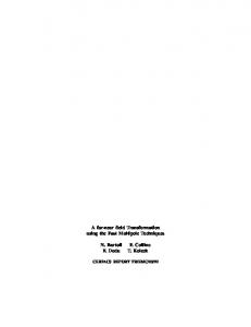
A key concept in understanding the algorithm is that of wellseparatedness. A point or cell is said to be well-separated from a cell C if it lies outside the domain of C and C ’s colleagues (colleagues are defined as the cells of the same size as C that are adjacent to C ). Using this concept, the FMM translates Newton’s insight into the following: If a point P is well-separated from a cell C , then C can be represented by a multipole expansion about its center as far as P is concerned. The force on P due to particles within C is computed by simply evaluating C ’s multipole expansion at P , rather than by computing the forces due to each particle within C separately. The same multipole expansion, computed once, can be evaluated at several points, thus saving a substantial amount of computation. The multipole expansion of a cell is a series expansion of the properties of the particles within it (expansions of nonterminal cells are computed from the expansions of their children). It is an exact representation if an infinite number of terms is used in the expansion. In practice, however, only a finite number of terms, say m, is used, and this number determines the accuracy of the representation. Representing cells by their multipole expansions is not the only insight exploited by the FMM. If a point P (be it a particle or the center of a cell) is well-separated from cell C , then the effects of P on particles within C can also be represented as a Taylor series or local expansion about the center of C , which can then be evaluated at the particles within C . Once again, the effects of several such points can be converted just once each and accumulated into C ’s local expansion, which is then propagated down to C ’s descendants and evaluated at every particle within C . The mathematics of computing multipole expansions, translating them to local expansions, and shifting both multipole and local expansions are described in [7]. To exploit the above mechanisms for computing forces, the adaptive FMM associates with every cell C a set of four lists of cells. The cells in a list bear a certain spatial relationship to C with respect to well-separatedness. Some of these lists are defined only for leaf cells of the tree, while others are defined for internal cells as well. The lists for a leaf cell C are described in Figure 3, and their role is discussed in more detail in [7, 15]. Using these lists, the adaptive FMM proceeds in the following steps:
P
Q Q R R
P
Figure 1: A two-dimensional particle distribution and the corresponding quadtree. C
D
C’s desecendent
D’s desecendent
Leaf cells within C
Leaf cell within D
Figure 2: Computing forces on particles in cell D due to particles in cell C in the FMM. 1. Build Tree: The tree is built by loading particles into an initially empty root cell. 2. Construct Interaction Lists: The U , V and W lists are constructed explicitly. The X list is not constructed, since it is the dual of the W list. 3. Upward Pass: The multipole expansions of all cells are computed in an upward pass through the tree. Expansions of leaf cells are computed from the particles within them, and expansions of internal cells from those of their children. 4. Compute List Interactions: For every cell C , the relevant list interactions are computed. First, if C is a leaf, interactions between all particles in C are computed directly with all particles in C ’s U list. Second, the multipole expansions of all cells in the V list of C are translated and accumulated into local expansions about the center of C . Third, if C is a leaf, the multipole expansions of the cells in the W list of C are evaluated at the particles in C . Since the X list is the dual of the W list and does not need to be constructed explicitly, X list interactions are computed at the same time as the W list interactions in our implementations. That is, for every cell W i in its W list, C first computes the W list interaction and updates the forces on its own particles accordingly, and then computes the X list interaction and updates the local expansion of Wi . Since X list interactions are thus computed by leaf cells, internal cells compute only their V list interactions.
5. Downward Pass: The local expansions of internal cells are propagated down to the leaf cells in a downward pass through the tree. 6. Evaluate Local Expansions: For every leaf cell C , the resulting local expansion of the cell (obtained from the previous two steps) is evaluated at the particles within it. This resulting force on each particle is added to the forces computed in steps 3 and 6. The direct computation of interactions among internal cells is the key factor that distinguishes the FMM from the Barnes-Hut method, the other major hierarchical N-body method. In the Barnes-Hut method, forces are computed particle by particle. The tree is traversed once per particle to compute the forces on that particle, so that the only interactions are between a particle and another particle/cell. The use of cell-cell interactions allows the FMM to have a better asymptotic complexity, but is also responsible for complicating the partitioning techniques required to obtain good performance, as we shall see. Our example application iterates over several hundred timesteps, every time step executing the above steps as well as one more that updates the velocities and positions of the particles at the end of the time-step. For the problems we have run, almost all the sequential execution time is spent in computing list interactions. The majority of this time (about 60-70%) is spent in computing V list interactions, next U list (about 2030%) and finally the W and X lists (about 10%). Building the tree and updating the particle properties take less than 1% of the time in sequential implementations.
X V
X U
V
U
U
WW U U
c
List U (leaf cells only): all leaf cells adjacent to C. These cells cannot be approximated in any way .
X U
UW U WW
UW
U
U
V
V
V
V
V
V
X
List V (all cells): Children of the colleagues of C’s parent that are well−separated from C. These are well−separated from C but not from C’s parent. List W (leaf cells only): Descendants of C’s colleagues whose parents are adjacent to C, but which are not themselves adjacent to C. Multipole expansions of these cells can be evaluated at particles in C; their parents’ multipole expansions cannot; and their expansions cannot be translated to local expansions about C’s center List X (all cells): Dual of W list: cells such that C is in their W list. Their multipole expansions cannot be translated to C’s center, but their individual particle fields can.
Figure 3: Interaction lists for a cell in the adaptive FMM.
3 Taking Advantage of Parallelism 3.1
The Available Parallelism
All the phases in the FMM afford substantial parallelism., which we exploit in parallel programs written for a machine that supports a shared address space. We exploit paralleism only within a phase. Fine-grained overlap across phases can be exploited by synchronizing at the level of individual cells, but this can incur a lot of overhead without hardware support and is unlikely to be beneficial. Although the basic entities in the N-body problem are particles, the above description makes it clear that the preferred units of parallelism are cells in all phases of the FMM other than tree-building. The tree-building, as well as the upward and downward passes to transfer expansions, clearly require both communication and cell-level synchronization, since different processors may own a parent and its child. The cell-level synchronization required includes mutual exclusion in the tree-building phase, and event synchronization to preserve dependences between parents and their children in the upward and downward passes. These upward and downward passes also have limited parallelism at higher levels of the tree (close to the root), which may become an important performance limitation on very large-scale machines when the number of processors becomes large relative to the problem size. Some of the list interactions may require synchronization for mutual exclusion. For example, in a straightforward implementation a processor writes the U list and X list interaction results of cells that may not belong to it. This locking can be eliminated for the U list interactions, and can be reduced for X list interactions as follows: Instead of writing the X list interaction results into the cumulative local expansion of the target cell (which the owning processor of that cell also writes), a separate per-cell X list result data structure is maintained so that both it and the local expansion updates can be written without locking; this array is then accumulated into the local expansion only during the downward pass. In any event, the communication in the interaction phase has the important prop-
erty that the data read are not modified during this phase, but only later on in the update or upward pass phases, a property that can be taken advantage of by coherence and data transfer protocols, particularly since the interaction phase is the most time-consuming. Finally, the update phase can be performed without synchronization or communication.
3.2
Goals and Difficulties in Effective Parallelization
In general, there are six major sources of overhead that inhibit a parallel application from achieving effective speedups over the best sequential implementation: inherently serial sections, redundant work, overhead of managing parallelism, synchronization overhead, load imbalance and communication. As in many scientific applications, the first four are not very significant here. Let us therefore define the goals of our parallel implementations in the context of the last two sources. Load Balancing: The goal in load balancing is intuitive: Cells should be assigned to processors to minimize the time that any processor spends waiting for other processors to reach synchronization points. Data Locality: Modern multiprocessors are built with complex memory hierarchies, in which processors have faster access to data that are closer to them in the hierarchy. Exploiting the locality in data referencing that an application affords can increase the fraction of memory references that are satisfied close to the issuing processor, and hence improve performance. While we make all reasonable attempts to exploit locality within a processing node, we restrict our discussion of data locality to reducing the interprocessor communication in the application by scheduling tasks that access the same data on the same processor. We do not examine several other, more detailed issues related to locality 1 or the impact of locality in a network topology. Many scientific applications operate on uniform problem domains and use algorithms which directly require only local1 Such as prefetching data with long cache lines or in software, falsesharing of data, and cache mapping collisions.
ized communication (see, for example, [17]). This application, however, has several characteristics that complicate the task of obtaining effective parallel performance. In particular: � Direct, relatively unstructured, long-range communication is required in every time-step, although the use of hierarchy causes the amount of communication to fall off with distance from a particle/cell. � The physical domain in galactic simulations is typically highly nonuniform, which makes it difficult to balance the computation and the communication across processors. For example, the work done per unit of parallelism (cell) is not uniform, and depends on the entire spatial distribution. � The dynamic nature of the simulation causes the distribution of particles, and hence the cell structure and work/communication distributions, to change across timesteps. There is no steady state. This means that no static partitioning of particles or space among processors is likely to work well, and repartitioning is required every time-step or few time-steps. In fact, the natural units of parallelism (cells) do not even persist across times-steps— since both the bounding box and the particle distribution change—and therefore cannot be partitioned statically anyway. � The fact that communication falls off with distance equally in all directions implies that a processor’s partition should be spatially contiguous and not biased in size toward any one direction, in order to minimize communication frequency and volume. � The different phases in a time-step have different relative amounts of work associated with particles/cells, and hence different preferred partitions if viewed in isolation.
Before we discuss the techniques we use to obtain both data locality and load balancing despite these characteristics, let us first describe the multiprocessor environments we use in our experiments.
4 The Execution Platforms We perform experiments to evaluate the performance of our schemes on two parallel machines that provide a cachecoherent shared address space: the Stanford DASH multiprocessor, and the Kendall Square Research KSR-1. In addition, we use a simulated multiprocessor to extend our results to more processors and to obtain quantitative support for some of our architectural implications (such as inherent communication to computation ratio and working set size).
The Stanford DASH Multiprocessor The DASH multiprocessor is a state-of-the-art research machine [13]. The machine we use has 48 processors organized in 12 clusters. A cluster comprises 4 MIPS R3000 processors connected by a shared bus, and clusters are connected together in a mesh network. Every processor has a 64KB first-level cache memory and a 256KB second-level cache, and every cluster has an equal fraction of the physical memory on the machine. All caches in the system are kept coherent in hardware using a distributed directory-based protocol. A hit in the first level cache is satisfied in a single cycle, while references satisfied in the second
level cache and in local memory stall the issuing processor for 15 and 30 cycles, respectively. Misses that go remote take about 100 or 135 cycles, depending on whether or not the miss is satisfied on the node in which the memory for the referenced datum is allocated.
The Kendall Square Research KSR-1 The KSR-1 is a commercial example of a new kind of architecture called an ALLCACHE or Cache-only Memory Architecture (COMA). Like in more traditional cache-coherent architectures, a processing node has a processor, a cache and a “main memory”. The difference is that the main memory on the node is itself converted into a very large, hardware-managed cache, by adding tags to cache-line sized blocks in main memory. This large cache, which is the only “main memory” in the machine, is called the attraction memory (AM) [6]. The location of a data item in the machine is thus decoupled from its physical address, and the data item is automatically moved (or replicated) by hardware to the attraction memory of a processor that references it. A processing node on the KSR-1 consists of a single 20MHz custom-built processor, a 256 KB instruction cache, a 256 KB data cache, and a 32MB attraction memory [4]. The machine is configured as a hierarchy of slotted, packetized rings, with 32 processing nodes on each leaf-level ring. We use a two-ring machine, with 64 processors. Since a couple of the processors on each ring have to perform system functions and are therefore slower than the others, we present results on only upto 60 processors. Reference latencies are as follows: 2 cycles to the subcache, 20 cycles to the AM, 150 cycles to a remote node on the local ring, and 570 cycles to another ring. The line size in the data subcache is 64 bytes, while that in the AM (which is the unit of data transfer in the network) is 128 bytes. The unit of data allocation in the AMs, called a page, is 16KB. The processor on the KSR-1 is rated lower than the DASH processor for integer code, but is much faster in peak operation on floating point code (40 MFlops versus 8 MFlops). KSR-1 also has higher interprocessor communication latency (both in processor cycles and in actual time, see above), but higher peak communication bandwidth owing to its longer cache line size.
The Simulated Multiprocessor The real multiprocessors that we use have the limitations of having only a certain number of processors, and of distorting inherent program behavior owing to their specific memory system configurations. To overcome these limitations we also run our programs on a simulator of an idealized shared-memory multiprocessor architecture [6]. The timing of a simulated processor’s instruction set is designed to match that of the MIPS R3000 CPU and R3010 floating point unit. Every processor forms a cluster with its own cache and equal fraction of the machine’s physical memory. A simple three-level non-uniform memory hierarchy is assumed: hits in the issuing processor’s cache cost a single processor cycle; read misses that are satisfied in the local memory unit stall the processor for 15 cycles, while those that are satisfied in some remote cluster (cache or memory unit) stall it for 60 cycles; since write miss latencies can be hidden more easily by software/hardware techniques, the corresponding numbers for write misses are 1 and 3 cycles, respectively.
5 Obtaining Effective Parallel Performance We have seen that it is not straightforward to obtain both load balancing and data locality simultaneously in this application. Whatever the technique used to partition cells for physical locality, the relative amounts of work associated with different cells must be known if load balancing is to be incorporated in the partitioning technique without resorting to dynamic task stealing (which has its own overheads and compromises locality). Let us therefore first discuss how we determine the work associated with a cell, and then describe the techniques we use to provide locality.
5.1
Determining the Work Associated with Cells
There are two problems associated with load balancing in this application. First, the naive assumption that every cell has an equal amount of work associated with it does not hold. Different childless cells have different numbers of particles in them, and different cells (childless or parent) have interaction lists of different sizes depending on the density and distribution of particles around them. The solution to this problem is to associate a cost with every cell, determined by the amount of computation needed to process its interactions. The second problem is that the cost of a cell is not known a priori, and changes across time-steps. In fact, even the cells themselves do not persist across time-steps, since both the bounding box and the tree structure change. Let us first ignore the latter problem and see how we would determine the changing cell costs if cells did persist across time-steps, and then take care of the lack of cell persistence. There is a key insight into N-body application characteristics that allows us to estimate cell costs even though the costs change across time-steps. Since N-body problems typically simulate physical systems that evolve slowly with time, the distribution of particles changes very slowly across consecutive time-steps, even though the change from the beginning to the end of the simulation may be dramatic. In fact, large changes from one time-step to the next imply that the timestep integrator being used is not accurate enough and a finer time-step resolution is needed. This slow change in distribution suggests that the work done to process a cell’s interactions in one time-step is a good measure of its cost in the next timestep. All we therefore need to do is keep track of how much computation is performed when processing a cell in the current time-step. In the Barnes-Hut method, the interactions that a particle computes are very similar, so that it suffices to count the number of interactions and use that count as an estimate of the particle’s cost. In the FMM, however, a cell computes different types of interactions with cells in different interaction lists. It doesn’t suffice to measure cost as simply the number of interactions per cell, or even the number of interactions of different types. Instead, for each type of interaction, we precompute the costs—in cycle counts—of certain primitive operations whose costs are independent of the particular interacting entities. Since the structure of every type of interaction is known, the cycle count for a particular interaction is computed by a very simple function for that type of interaction, parametrized by
the number of expansion terms being used and/or the number of particles in the cells under consideration. The cost of a leaf cell is the sum of these counts in all interactions that the cell computes. The work counting is done in parallel as part of the computation of cell interactions, and its cost is negligible. Let us now address the problem that cells not persist across time-steps, so that it doesn’t really make sense to speak of using a cell’s cost in one time-step as an estimate of its cost in the next time-step 2. To solve this problem, we have to transfer a leaf cell’s cost down to its particles (which do persist across time-steps) and then back up to the leaf cell that contains those particles in the next time-step. We do this as follows. The profiled cost of a leaf cell is divided equally among its particles. In the next time-step, a leaf cell examines the costs of its particles, finds the cost value that occurs most often, and multiplies this value by its number of particles to determine its cost. Since internal cells only compute V list interactions in our implementations (see Section 2.1), and since the cost of a V list interaction depends only on a program constant (the number of terms used in the expansions) and not on the number of particles in any cell, the cost of an internal cell is simply computed from the number of cells in its V list in the new time-step.
5.2
Partitioning for Locality and Load Balancing
As mentioned earlier, the goal in providing locality is that the cells assigned to a processor should be close together in physical space. Simply partitioning the space statically among processors is clearly not good enough, since it leads to very poor load balancing. In this subsection, we describe two partitioning techniques that try to provide both locality and load balancing, both of which use the work-counting technique of the previous subsection. The first technique partitions the computational domain space directly, while the second takes advantage of an insight into the application’s data structures to construct a more cost-effective technique. Since the particle distribution and hence the cell structure changes dynamically, the partitioning is redone every time-step.
5.2.1
Partitioning Space: Orthogonal Recursive Bisection
Orthogonal Recursive Bisection (ORB) is a technique for providing physical locality in a problem domain by explicitly partitioning the domain space [5]. The idea here is to recursively divide space into two subspaces with equal costs, until there is one subspace per processor (see Figure 7). Initially, all processors are associated with the entire domain space. Every time a space is divided, half the processors associated with it are assigned to each of the subspaces that result. The Cartesian direction in which division takes place is usually alternated with successive divisions, and a parallel median finder is used to determine where to split the current subspace in the direction chosen for the split. ORB was first used for hierarchical N-body problems by Salmon [14], in a message-passing implementation of a galactic simulation using the Barnes-Hut 2 This is a problem that the Barnes-Hut method does not have, for example, since work is associated with particles rather than cells in that case, and particles persist across time-steps.
method. The partitioning in that case was made simpler by the fact that work in the Barnes-Hut method is associated only with particles and not with cells. Particles are naturally represented by points, and can be partitioned cleanly by ORB bisections since they fall on one or the other side of a bisecting line. Further details of implementing ORB are omitted for reasons of space, and can be found in [15, 14]. ORB introduces several new data structures, including a separate binary ORB tree of recursively subdivided subdomains. The fact that work is associated with internal cells as well in the FMM (rather than just leaves) requires that we include internal cells in determining load balancing, which is not necessary in Barnes-Hut. Also, besides the leaf or internal cell issue, the fact that the unit of parallelism is a cell rather than a particle complicates ORB partitioning in the FMM. When a space is bisected in ORB, several cells (leaf and internal) are likely to straddle the bisecting line (unlike particles, see Figure 4). In our first implementation, which we call ORB-initial, we try to construct a scheme that directly parallels the ORB scheme used in [14] for Barnes-Hut (except that internal cells are included among the entities to be partitioned). Cells, both leaf and internal, are modeled as points at their centers for the purpose of partitioning, just as particles are in the Barnes-Hut method. At every bisection in the ORB partitioning, therefore, a cell that straddles the bisecting line (called a border cell) is given to whichever subspace its center happens to be in. As our performance results will show, this treatment of border cells in the ORB-initial scheme leads to significant load imbalances. It is not difficult to see why. Given the fact that cells are always split in exactly the same way (into four children of equal size), the centers of many cells are likely to align exactly with one another in the dimension being bisected. These cells are in effect treated as an indivisible unit when finding a bisector. If a set of these cells straddles a bisector, as is very likely, this entire set of border cells will be given to one or the other side of the bisector (see Figure 4(a)), potentially giving one side of the bisector a lot more work than the other. 3 The significant load imbalance thus incurred in each bisection may be compounded by successive bisections. To solve this problem, we extend the ORB method as follows. Once a bisector is determined (by representing all cells as points at their centers, as before), the border cells that straddle the bisector are identified and repartitioned. In the repartitioning of border cells, we try to equalize costs as far as possible while preserving the contiguity of the partitions (see Figure 4(b)). A target cost for each subdomain is first calculated as half the total cost of the cells in both subdomains. The costs of the border cells are then subtracted from the costs of the subdomains that ORB-initial assigned them to. Next, the border cells are visited in an order sorted by position along the bisector, and assigned to one side of the bisector until that side reaches the target cost. Once the target cost is reached, the rest of the border cells are assigned to the other side of the bisector. We call this scheme that repartitions border boxes ORB-final. 3 This situation is even more likely with a uniform distribution, where many cells will have their centers exactly aligned in the dimension along which a bisection is to be made.
5.2.2
A Simpler Partitioning Technique: Costzones
Our costzones partitioning technique takes advantage of another key insight into the hierarchical N-body methods, which is that they already have a representation of the spatial distribution encoded in the tree data structure they use. We therefore partition the tree rather than partition space directly. In the costzones scheme, the tree is conceptually laid out in a twodimensional plane, with a cell’s children laid out from left to right in increasing order of child number. Figure 5 shows an example using a quadtree. The cost of (or work associated with) every cell, as counted in the previous time-step, is stored with the cell. Every internal cell holds the sum of the costs of all cells (leaf or internal) within it plus its own cost 4 . In addition, it holds its own cost separately as well. The total cost in the domain is divided among processors so that every processor has a contiguous, equal range or zone of costs. For example, a total cost of 1000 would be split among 10 processors so that the zone comprising costs 1-100 is assigned to the first processor, zone 101-200 to the second, and so on. Which cost zone a cell belongs to is determined by the total cost up to that cell in an inorder traversal of the tree. Code describing the costzones partitioning algorithm is shown in Figure 6. Every processor calls the costzones routine with the Cell parameter initially being the root of the tree. The variable cost-to-left holds the total cost of the particles that come before the currently visited cell in an inorder traversal of the tree. Other than this variable, the algorithm introduces no new data structures to the program. In the traversal of the planarized tree that performs costzones partitioning, a processor examines cells for potential inclusion in its partition in the following order: the first two children (from left to right), the parent, and the next two children 5 . The algorithm requires only a few lines of code, and has negligible runtime overhead, as we shall see. The costzones technique yields partitions that are contiguous in the tree as laid out in a plane. How well this contiguity in the tree corresponds to contiguity in physical space depends on the orderings chosen for the children of all cells when laying them out from left to right in the planarized tree. The simplest ordering scheme—and the most efficient for determining which child of a given cell a particle falls into—is to use the same ordering for the children of every cell. Unfortunately, there is no single ordering which guarantees that contiguity in the planarized tree will always correspond to contiguity in physical space. The partition assigned to processor 3 in Figure 7 illustrates the lack of robustness in physical locality resulting from one such simple ordering in two dimensions (clockwise from the bottom left child for every node). While all cells within a tree cell are indeed in the same cubical region of space, cells (subtrees) that are next to each other in the linear ordering from left to right in the planarized tree may not have a common ancestor until much higher up in the tree, and may therefore not be anywhere near each other in physical space. 4 These cell costs are computed during the upward pass through the tree that computes multipole expansions. 5 Recall that we use a two-dimensional FMM, so that every cell has at most four children.
Box goes to the right
Box goes to the left
(b) ORB-final
(a) ORB-initial
Figure 4: Partitioning of border cells in ORB for the FMM.
Proc 1
Proc 2
Proc 3
Proc 4
Proc 5
Proc 6
Proc 7
Proc 8
Figure 5: Tree partitioning in the costzones scheme. There is, however, a simple solution that makes contiguity in the planarized tree always correspond to contiguity in space. In this solution, the ordering of children in the planarized tree is not the same for all cells. However, the ordering of a cell C ’s children is still easy to determine, since it depends on only two things: the ordering of C ’s parent’s children (i.e. C’s siblings), and which child of its parent C is in that ordering. Consider a two-dimensional example. Since every cell has four children in two dimensions, there are eight ways in which a set of siblings can be ordered: There are four possible starting points, and two possible directions (clockwise and anticlockwise) from each starting point. It turns out that only four of the eight orderings need actually be used. Figure 8(a) shows the four orderings we use in our example, and illustrates how the ordering for a child is determined by that for its parent. The arrow in a cell represents the ordering of that cell’s children. For example, if the children are numbered 0, 1, 2, 3 in a counterclockwise fashion starting from the upper right, then in case (1) in Figure 8(a) the children of the top-level cell are ordered 2, 1, 0, 3, and in case (2) the children are ordered 2, 3, 0, 1. The ordering of the children’s children are also shown. Figure 8(b) shows the resulting partitions given the same distribution as in Figure 7. The bold line follows the numbering order, starting from the bottom left cell. All the partitions are physically contiguous in this case. The three-dimensional case is handled the same way, except that there are now 32 different orderings used instead of 4. A discussion of the extension to three-dimensions can be found in [15]. We use this more robust, nonuniform child ordering method in the partitioning scheme we call costzones.
5.3
Results
Figure 9 shows the performance results on DASH for a simulation of two interacting Plummer model [1] galaxies that start out slightly separated from each other. The results shown are for 32K particles and an accuracy of 10010, which translates to m=39 terms in the expansions. Five time-steps are run, of which the first two are not measured to avoid cold-start effects that would not be significant in a real run over many hundreds of time-steps. Clearly, both the ORB-final and costzones schemes achieve very good speedups. The ORB-initial scheme is significantly worse than the ORB-final scheme, which shows that the extension to handle border boxes intelligently—rather than treat them as particles at their centers—is important. To demonstrate that it is also important to take the cost of internal cells into account when partitioning, the figure also shows results for a scheme called costzones-noparents, in which only the cost of leaves is taken into account during partitioning and internal cells are simply assigned to the processor that owns most of their children for locality. While both the ORB-final and costzones schemes perform very well upto 32 processors (ORB requires the number of processors to be a power of two and therefore cannot be used with 48 processors), we can already see that costzones starts to outperform ORB. This difference is found to become larger as more processors are used, as revealed by experiments with more processors on the simulated multiprocessor. Closer analysis and measurement of the different phases of the application reveals the reasons for this (see Figure 10). One reason is that the costzones scheme does provide a little better load balancing and hence speeds up the force-computation a little better. However, the main reason is that the ORB partitioning phase
Costzones (Cell,cost-to-left) f if (Cell is a leaf) f if (Cell is in my range) add Cell to my list g else f for (first two Children of Cell) f if (cost-to-left < max value of my range) f if (cost-to-left + Child cost >= min value of my range) Costzones (Child,cost-to-left) cost-to-left += Child cost g g if (cost-to-left is in my range) f add Cell itself to my list cost-to-left += cost of Cell itself g for (last two Children of Cell) f if (cost-to-left < max value of my range) f if (cost-to-left + Child cost >= min value of my range) Costzones (Child,cost-to-left) cost-to-left += Child cost g g g g
22
23
26
27
38
39
42
43
21
24
25
28
37
40
41
44
20
19
30
29
36
35
46
45
17
18
31
32
33
34
47
48
16
13
12
11
54
53
52
49
15
14
9
10
55
56
51
50
2
3
8
7
58
57
62
63
1
4
5
6
59
60
61
64
Figure 6: Costzones-final partitioning for the FMM
(1)
(2) 22
ORB
27
38
39
42
43
23
26
21
24
25
28
37
40
41
44
18
19
30
31
34
35
46
47
17
20
29
32
33
36
45
48
6
7
10
11
54
55
58
59
5
8
9
12
53
56
57
60
2
3
14
16
50
51
62
63
1
4
13
15
49
52
61
64
Costzones: Uniform numbering
A split partition assigned to the same processor
(3)
(4) Proc 1
Proc 2
Proc 3
Proc 4 Proc 5 Proc 6 Proc 7
Proc 8
(a)Figure Ordering cells 7: ORB and of costzones with uniform numbering. itself is more expensive than costzones partitioning (as the descriptions earlier in this section should show), the difference in partitioning cost increasing with the number of processors. The cost of costzones partitioning grows very slowly with n or p, while that of ORB grows more quickly. Thus, the costzones scheme is not only much simpler to implement, but also results in better performance, particularly on larger machines. In addition to the nonuniform distribution described above,
(b) The resulting partitions
42.0
|
24.0
|
18.0
|
12.0
|
��
� ��
��
� �� �� � �� �
|
6.0
�
�
|
30.0
� DASH, eps = 1e-10
DASH, eps = 1e-6 � KSR, eps = 1e-10 � KSR, eps = 1e-6
|
36.0
5.3.1
ideal
�
� �
�� �
|
0.0 | 0
|
|
|
|
|
|
|
|
6
12
18
24
30
36
42
48
Number of Processors
48.0
� DASH, eps = 1e-10
DASH, eps = 1e-6 � KSR, eps = 1e-10 � KSR, eps = 1e-6
�
|
18.0
|
12.0
|
� ��
� �� �� � �� �
|
|
|
|
|
|
|
|
6
12
18
24
30
36
42
48
Number of Processors
10.0
8.0
6.0
4.0
� Old Tree Build � New Tree Build
�
�
� � � |
2.0
0.0 | 0
|
tions on both DASH and KSR-1. As expected, higher numbers of particles and greater force-calculation accuracies lead to slightly better speedups, particularly since both these lead to relatively more time being spent in the well-balanced phase of computing interactions. The difference between costzones and ORB partitioning is also emphasized as the force-calculation accuracy decreases (results not shown), since the impact of partitioning cost (which is independent of accuracy) becomes greater relative to the cost of computing interactions. Finally, we find that the speedups on DASH are consistently better than those on KSR-1. This is because the communication latencies are higher on KSR-1, and its ALLCACHE nature gives it no real advantages since the important working set of the application is very small and fits in the cache on DASH as well. Uniprocessor performance is also better on DASH by about 25%, primarily since there is a lot of integer code in the tree and list manipulations, and the processor on DASH does better on these. A more detailed discussion of DASH versus KSR-1 can be found in another paper in these proceedings [11].
� �
|
Figure 12: Speedups for the FMM application on DASH and KSR-1 (n = 32k).
12.0
|
|
Because the costzones and ORB partitioning techniques give every processor a contiguous partition of space, they effectively divide up the tree into distinct sections and assign a processor to each section. This means that once the first few levels of the tree are built, there is little contention for locks in constructing the rest of the tree, since processors then construct their sections without much interference. Most of the contention in the initial parallel tree-building algorithm outlined above is due to many processors simultaneously trying to update the first few levels of the tree.
|
�� �
|
0.0 | 0
The obvious way to parallelize the tree-building algorithm is to have processors insert their particles into the shared tree concurrently, synchronizing as necessary. This can lead to substantial locking overhead in acquiring mutually exclusive access whenever a processor wants to add a particle to a leaf cell, add a child to an internal cell, or subdivide a leaf cell.
|
|
24.0
��
� ��
Figure 10 also reveals a potential bottleneck to performance on large parallel machines, which is that the tree-building phase does not speed up as well in parallel as force-computation. If the number of particles per processor stays very large, tree building is not likely to take much time relative to the rest of the time-step computation. However, under the most realistic methods of time-constrained scaling, the number of particles per processor shrinks as larger problems are run on larger machines [16], and tree-building can become a significant part of overall execution time.
|
30.0
6.0
ideal
�
� �
|
36.0
|
42.0
|
Speedup
Figure 11: Speedups for the FMM application on DASH and KSR-1 (n = 64k).
The Parallel Tree-Building Bottleneck
% Time Spent in TreeBuild
|
Speedup
48.0
�
�
�
�
�
�
|
|
|
|
|
|
8
16
24
32
40
48
Number of Processors
Figure 13: Percentage of total execution time spent building the tree on DASH. Fortunately, the same physical locality in our partitions that helps the intial parallel tree-building algorithm also allows us to construct a better algorithm. It is possible to substantially reduce both the contention at the upper levels of the tree and the amount of locking of cells that needs to be done, by splitting the parallel tree construction into two steps. First, every processor builds its own version of the tree using only its own particles. The root of this local tree represents the whole computational domain, not just a domain large enough to hold the local particles. This step is made more efficient by having a processor remember where in its tree it inserted its last
particle, and start traversing the tree from there for the next particle, rather than from the root. No locking is needed in this step. Second, these individual trees are merged together into the single, global tree used in the rest of the computation. Since the root cells of all the local trees represent the entire computational domain, a cell in one tree represents the same subspace as the corresponding cell in another tree. This fact allows the merge procedure to make merging decisions based on the types of the cells in the local and global trees only (i.e. whether the cell is internal cell or a leaf etc.). The merge procedure starts at the root of both trees, comparing the type of cell (body, cell, or empty) from each tree, and taking an appropriate action based on the two types. There are six possible cases: 1. local cell is internal, global cell is empty: The local cell is inserted into the tree. 2. local cell is internal, global cell is a leaf: The global cell is removed from the tree. Then the global particle is inserted into the subtree with the local cell as the root. The parent of the global cell is relocked, and the local cell is inserted into the tree. 3. local cell is internal, global cell is internal: A spatial equivalent to the local cell already exists in the global tree, so nothing is done with the local cell. The merge algorithm is recursively called on each of the local cell’s children and their counterparts in the global tree. 4. local cell is a leaf, global cell is empty: Same as Case 1. 5. local cell is a leaf, global cell is a leaf: Same as Case 2. 6. local cell is a leaf, global cell is internal: The local cell is subdivided, pushing the particle one level deeper in the local tree. Since the local cell is now internal, Case 3 applies. Details of the algorithm and pseudocode can be found in [15]. The algorithm greatly alleviates the problem of too much contention at the early levels of the tree. When the first processor tries to merge its tree into the global tree, it finds the global root null. By case 1, it sets the global root to its root. The processor’s local tree has now become the global tree, and its size reduces contention at any one cell. Just as important, it only took one locking operation to merge the entire first local tree. Since large subtrees are merged in a single operation, rather than single particles, the amount of locking required (and hence both the overhead of locking as well as the contention) is greatly reduced. The reduction in locking overhead and contention comes at a cost in redundant work. There is some extra work done in first loading particles into local trees and then merging the local trees, rather than loading particles directly into the global tree (as in the old tree building algorithm). When the partitioning incorporates physical locality, this extra work overhead is small and the reduction in locking overhead is substantial, since large subtrees are merged in a single operation. Of course, if the partitioning does not incorporate physical locality, this new tree-building algorithm has no advantages over the old one,
and the extra work overhead it introduces will make it perform significantly worse. To compare the old and new tree-building algorithms, Figure 13 shows the percentage of the total execution time of the application on the DASH multiprocessor that is spent in building the tree. The problem size used is the same as the one for which speedups are presented in Figure 9. The new algorithm clearly performs much better than the old one, particularly as the number of processors increases.
6 Summary and Architectural Implications We have shown that despite their nonuniform and dynamically changing characteristics, N-body simulations that use the adaptive Fast Multipole Method can be partitioned and scheduled for effective parallel performance on shared-address-space machines. We described a method for obtaining load balancing without resorting to dynamic task stealing, and proposed and evaluated two partitioning techniques, both of which use this load balancing method but use different techniques for providing data locality. We showed that our costzones partitioning technique provides better performance than an extended recursive bisection technique—particularly on larger numbers of processors—by taking advantage of an additional insight into the Fast Multipole Method. Using the costzones technique, we demonstrated 45-fold speedups on the Stanford DASH multiprocessor, even for a relatively small problem size. In addition to understanding how to parallelize important classes of applications, it is also important to understand the implications of application characteristics for the design of parallel systems. We have studied several of these implications for the FMM. Our methodology and detailed results can be found in [16, 15]. Here, we summarize the main results. We found that exploiting temporal locality by caching communicated data is critical to obtaining good performance, and that hardware caches on shared-address-space machines are well-suited to providing this locality automatically and efficiently. On the other hand, data distribution in main memory, to allocate the particle/cell data assigned to a processor in that processor’s local memory unit, is both very difficult to implement and not nearly as important. We also found that the nonuniform, dynamically changing nature of the application causes implicit communication through a shared address space to have substantial advantages over explicit communication through message-passing in both ease of programming and performance. Finally, we examined how some important application characteristics scale as larger problems are run on larger parallel machines. We showed that scaling to fill the memory on the machine in unrealistic since it increases the execution time too much, and that the following results hold under the most realistic, time-constrained scaling model: (i) the main memory requirements (or number of particles) per processor become smaller, (ii) the communication to computation ratio increases slowly, but is small enough in absolute terms to allow good performance even on large-scale machines, and (iii) the working set size per processor, which helps determine the ideal cache size for the computation, also grows slowly but is very small.
In fact, the important working set holds roughly the amount of data reused from one cell’s list interactions to another’s, and is therefore independent of the number of particles and the number of processors; it depends only on the number of terms used in the multipole expansions, which grows very slowly with problem and machine size. As a result, unless overheads and load imbalances in the phases of computation (such as the tree building phase, discussed earlier, and the load-imbalanced upward and downward passes through the tree) that are not significant on the problem and machine sizes available today become significant on much larger machines, machines with large numbers of processors and relatively small amounts of cache and main memory per processor should be effective in delivering good performance on applications that use the adaptive Fast Multipole Method.
Acknowledgements We would like to thank Leslie Greengard for providing us with the sequential program and for many discussions. This work was supported by DARPA under Contract No. N00039-91-C0138. Anoop Gupta is also supported by a Presidential Young Investigator Award, with matching grants from Ford, Sumitomo, Tandem and TRW.
References [1] S.J. Aarseth, M. Henon, and R. Wielen. Astronomy and Astrophysics, 37, 1974. [2] Andrew A. Appel. An efficient program for many body simulation. SIAM Journal of Scientific and Statistical Computing, 6:85–93, 1985. [3] Joshua E. Barnes and Piet Hut. A hierarchical O(N log N) force calculation algorithm. Nature, 324(4):446–449, 1986. [4] A. J. Chorin. Numerical study of slightly viscous flow. Journal of Fluid Mechanics, 57:785–796, 1973. [5] Geoffrey C. Fox. Numerical Algorithms for Modern Parallel Computer Architectures, chapter A Graphical Approach to Load Balancing and Sparse Matrix Vector Multiplication on the Hypercube, pages 37–62. SpringerVerlag, 1988. [6] Stephen R. Goldschmidt and Helen Davis. Tango introduction and tutorial. Technical Report CSL-TR-90-410, Stanford University, 1990. [7] Leslie Greengard. The Rapid Evaluation of Potential Fields in Particle Systems. ACM Press, 1987. [8] Leslie Greengard and William Gropp. Parallel Processing for Scientific Computing, chapter A Parallel Version of the Fast Multipole Method, pages 213–222. SIAM, 1987. [9] Leslie Greengard and Vladimir Rokhlin. A fast algorithm for particle simulation. Journal of Computational Physics, 73(325), 1987. [10] P. Hanrahan, D. Salzman, and L. Aupperle. A rapid hierarchical radiosity algorithm. In Proceedings of SIGGRAPH, 1991.
[11] John L. Hennessy Jaswinder Pal Singh, Truman Joe and Anoop Gupta. An empirical comparison of the ksr-1 allcache and stanford dash multiprocessors. In Supercomputing ’93, November 1993. [12] Jacob Katzenelson. Computational structure of the Nbody problem. SIAM Journal of Scientific and Statistical Computing, 10(4):787–815, 1989. [13] Dan Lenoski, James Laudon, Kourosh Gharachorloo, Anoop Gupta, and John Hennessy. The directory-based cache coherence protocol for the DASH multiprocessor. In Proceedings of the 17th Annual International Symposium on Computer Architecture, pages 148–159, May 1990. [14] John K. Salmon. Parallel Hierarchical N-body Methods. PhD thesis, California Institute of Technology, December 1990. [15] Jaswinder Pal Singh. Parallel Hierarchical N-body Methods and their Implications for Multiprocessors. PhD thesis, Stanford University, February 1993. [16] Jaswinder Pal Singh, Anoop Gupta, and John L. Hennessy. Implications of hierarchical N-body techniques for multiprocessor architecture. Submitted to ACM Transactions on Computer Systems. Early version available as Stanford Univeristy Tech. Report no. CSL-TR-92-506, January 1992. [17] Jaswinder Pal Singh and John L. Hennessy. High Performance Computing II, chapter Data Locality and Memory System Performance in the Parallel Simulation of Ocean Eddy Currents, pages 43–58. North-Holland, 1991. Also Stanford University Tech. Report No. CSL-TR-91-490. [18] Jaswinder Pal Singh, Chris Holt, Takashi Totsuka, Anoop Gupta, and John L. Hennessy. Load balancing and data locality in hierarchical N-body methods. Journal of Parallel and Distributed Computing. To appear. Preliminary version available as Stanford Univeristy Tech. Report no. CSL-TR-92-505, January 1992. [19] Feng Zhao. An O(n) algorithm for three-dimensional Nbody simulations. Technical Report 995, MIT Artificial Intelligence Laboratory, 1987.