An adaptive fast multipole accelerated Poisson solver for complex ...

An adaptive fast multipole accelerated Poisson solver for complex geometries T. Askham, A.J. Cerfon Courant Institute of Mathematical Sciences, New York University, New York, NY 10012

arXiv:1610.00823v1 [math.NA] 4 Oct 2016

Abstract We present a fast, direct and adaptive Poisson solver for complex two-dimensional geometries based on potential theory and fast multipole acceleration. More precisely, the solver relies on the standard decomposition of the solution as the sum of a volume integral to account for the source distribution and a layer potential to enforce the desired boundary condition. The volume integral is computed by applying the FMM on a square box that encloses the domain of interest. For the sake of efficiency and convergence acceleration, we first extend the source distribution (the right-hand side in the Poisson equation) to the enclosing box as a C 0 function using a fast, boundary integral-based method. We demonstrate on multiply connected domains with irregular boundaries that this continuous extension leads to high accuracy without excessive adaptive refinement near the boundary and, as a result, to an extremely efficient “black box” fast solver. Keywords: Poisson equation, Fast Multipole Method, Quadrature by Expansion, integral equations 1. Introduction The solution of the Poisson equation is a critical task in many areas of computational physics. The corresponding solvers need to be able to handle complex, multiply connected geometries, to be fast, adaptive, and to yield high order accuracy. Speed is of particular importance when the Poisson equation is part of a larger system of equations or in the inner loop of an optimization process. And since the physical quantity of interest is often the gradient of the solution, rather than the solution itself [2, 3, 4, 5, 6], partial derivatives of the solution must be computable with high accuracy as well. Integral equation techniques have the potential to address all the challenges mentioned above. Complex geometries may be handled by decomposing the solution to Poisson’s equation as the sum of a particular solution v that does not satisfy the proper boundary condition in general, plus a homogeneous solution uH that solves Laplace’s equation and is chosen so that the full solution u = v + uH satisfies the proper boundary condition. Fast and accurate solvers can be designed based on this construction. Indeed, several efficient and accurate integral equation based schemes exist to compute the solution of Laplace’s equation on complex geometries [7, 9, 10], and fast and accurate evaluation of the particular solution v on fully adaptive grids by use of the Fast Multipole Method (FMM) has also been demonstrated for Poisson’s equation [11, 12]. Furthermore, in integral equation formulations derivatives do not have to be computed through direct numerical differentiation. Instead, one can analytically differentiate the kernels in the integral representation of the solution, and thus obtain integral representations for the Preprint submitted to Journal of Computational Physics

October 5, 2016

derivatives of the solution as well. As a result the numerical error for the derivatives often converges at the same rate as the error for the solution itself [5, 12]. Remarkably, despite all the strengths described above, we are not aware of an integral equation based Poisson solver for planar problems that combines all the features at once. In [11, 13], grid adaptivity and FMM acceleration are demonstrated, but only simple geometries are considered. In contrast, in [14], Poisson’s equation is solved for complex geometries and with FMM-accelerated quadratures, but the solver relies on fast methods for uniform grids [15, 16]. The purpose of this manuscript is to close this gap and to present an adaptive, FMM-accelerated Poisson solver for complex geometries. We achieve this in the following way. We embed the irregular domain Ω on which Poisson’s equation needs to be solved in a larger square domain ΩB . We decompose the solution to Poisson’s equation as u = v + uH , and compute the particular solution v on ΩB with a fast and accurate solver for square domains [11]. In order to calculate v in this way, we need to extend the source function f on the right-hand side of Poisson’s equation beyond the domain Ω where it is originally given. We show that global function extension for f , constructed by solving Laplace’s equation or a higher order partial differential equation on the domain R2 \ Ω, leads to a robust, efficient and accurate algorithm for the evaluation of v. This idea is very similar in spirit to the extension technique recently presented by Stein et al.[18] for the immersed boundary method, but quite different in its implementation. Our approach for computing uH is standard in its formulation [19], but it relies on numerical tools developed recently for optimized performance. Specifically, we represent uH as a layer potential whose density solves a second-kind integral equation. We use generalized Gaussian quadrature [33, 34] to approximate the integrals, a fast direct solver [25] to compute the density and an FMM accelerated Quadrature By Expansion (QBX) algorithm [21] to evaluate uH inside Ω. The structure of the article is as follows. In Section 2 we present our formulation for the solution to Poisson’s equation, which is based on standard potential theory. We stress its computational challenges, which are then addressed in the following sections. In section 3, we describe an efficient and accurate algorithm for the evaluation of the particular solution v and its derivatives in a square box. While this algorithm plays a central role in our approach to the problem, the section is relatively brief because our solver relies on an implementation of the algorithm and techniques that have been discussed in detail elsewhere [11, 12]. In section 4, we explain how we use a global function extension algorithm in combination with a box Poisson solver for the computation of the particular solution v on the whole square domain ΩB . This is a key element of our solver, which allows us to deal with complex geometries in an efficient manner. In Section 5, we present our numerical method for calculating the homogeneous solution uH , as well as the function extension. Both are expressed as layer potentials and are computed in very similar ways. In Section 6 we study the performance of our new solver for two Poisson problems on a multiply connected domain. We summarize our work in Section 7 and suggest directions for future work. 2. The Potential Theoretic Approach to Poisson’s Equation In this article, we consider the solution u to Poisson’s equation with Dirichlet boundary conditions given by ∆u = f in Ω u = g on ∂Ω 2

(1) (2)

where Ω is a smooth planar domain, which may or may not be multiply connected. The standard potential theory-based approach to the solution of (1– 2) proceeds as follows. The first step is to calculate a particular solution, i.e. a function v which satisfies only equation (1) but does in general not satisfy equation (2). A natural candidate for v is given by Z v(x) = G(x, y)f (y) dy, (3) Ω

where G(x, y) is the free-space Green’s function for Poisson’s equation. For planar problems, G(x, y) = log(||x − y||)/2π. This is the situation we will consider in this article. Once v has been computed, the second step is to compute a homogeneous solution with appropriate boundary conditions. Specifically, one solves the following Dirichlet problem ∆uH = 0 in Ω H

u = g − v|∂Ω on ∂Ω.

(4) (5)

The solution to (1–2) is then the sum, u = v + uH . There are many options for the numerical implementation of these two steps and we will not attempt to provide an exhaustive review of them here. Instead, we focus on our new approach, which is designed to address situations for which the domain Ω may be irregular and where derivatives of the solution are also required with high accuracy. The purpose of this section is to give a short overview of our approach. This overview is divided into two subsections: subsection 2.1 concerns the computation of v, and subsection 2.2 describes the computation of uH . The presentation in these two subsections is meant to give a general idea of our numerical scheme, and is brief on purpose. We provide detailed descriptions of our numerical methods to calculate of v and uH in sections 3 and 4 for v, and section 5 for uH . 2.1. Computing the particular solution There are two challenges associated with the evaluation of the particular solution v through the integral (3). First, accurate quadratures must be used in order to handle the logarithmic singularity. Second, given a quadrature rule, the na¨ıve numerical approach to computing (3) would require O(N 2 ) work for a domain with N discretization nodes. It is now well known that the computational work can in fact be reduced to O(N ) via the fast multipole method [17]. Furthermore, for a fixed domain Ω, the quadrature rules for a weakly singular kernel G(x, y) can be precomputed using an adaptive, brute-force procedure [26]. As a result, there exist particularly efficient O(N ) algorithms, including optimized versions of the FMM [11], to compute the integral (3) for problems specified on a box. We choose such an algorithm for our solver, and provide some details of this type of method in Section 3. For irregular domains Ω, however, the situation is quite different. The calculation of appropriate quadratures is much more difficult and fewer optimizations of the FMM are available. A natural strategy, then, for irregular domains is to consider a larger, square domain ΩB containing Ω and to instead compute Z v(x) = G(x, y)fe (y) dy, (6) ΩB

where fe is defined on all of ΩB , and constructed such that fe = f on Ω. One of the main novelties of our work is to compute fe via global function extension: fe restricted 3

to R2 \ Ω is the solution of an elliptic partial differential equation with Dirichlet data fe = f on ∂Ω.The PDE is solved with a standard integral equation representation. We elaborate on this idea in Section 4. Remark 1. It should be noted here that the solution provided by any Poisson solver is a valid particular solution, though it will not necessarily be equal to the one given by (3). This includes in particular the solutions produced by FFT-based solvers for rectangular and circular domains, which are very fast in terms of work per grid point. The method of [14] uses such a particular solution, computed via Buneman’s method [27] and the modified stencils developed in [15]. The algorithm of [11], which we choose for our solver, is an alternative to such methods, with its greatest advantage being the ease with which it handles adaptive discretization. We demonstrate this advantage with numerical examples in Section 6. 2.2. Computing the homogeneous solution A standard approach to the solution of Laplace’s equation is to represent the solution H u as a layer potential with unknown density µ on the boundary. The representation should be chosen so that imposing the boundary conditions results in an invertible, second kind integral equation (SKIE) for the density on the boundary. This is a well-studied area and there exist appropriate integral representations for multiply connected domains [31, 29], unbounded domains [19], and for situations with other types of boundary conditions [30]. Further references can be found in the previously cited papers, and we recommend [19, 28] for very clear treatments of this topic. Once a suitable representation for uH is chosen, the discretization of the problem is then simply a matter of quadrature for the resulting SKIE. In general, the integral kernel may be singular and the choice of quadrature requires attention [20, 32, 21, 7, 33, 34]. Once discretized, there are many tools available for the fast solution of the resulting linear system, which we briefly discuss in Section 5. For this article, we choose a direct method [25] that is optimized for the type of problems considered here. After the density σ is computed, the solution uH can be evaluated in the domain. This step is trivially direct but it is not without its difficulties. With N discretization points in the domain and M discretization points on the boundary, na¨ıve computation of the necessary integrals would require O(M N ) work. This work can be reduced to O(M + N ) with the FMM. Because the integral kernel of the solution representation is typically singular in the ambient space (R2 ), computing the potential uH to high accuracy near the boundary requires special quadrature schemes. Such schemes have been developed recently [7, 21], and for our solver we choose to rely on the Quadrature By Expansion method (QBX) [21], which we also briefly discuss in section 5. 3. Box Codes This section reviews relevant features of the algorithm of [11], which is the original “box code”, and which we have implemented in our solver. By “box codes”, we mean a class of fast solvers which are used to evaluate integrals of the form Z V f (x) = G(x, y)f (y) dy , (7) Ω

where the integral kernel G(x, y) is a translation invariant Green’s function, the domain Ω is a box, and f (y) is a given density. We take G(x, y) = − log kx − yk/2π in what follows. 4

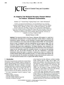
3.1. Outline of a box code As in all fast multipole methods, a FMM-based box code is based on a hierarchical division of space. Specifically, the domain is taken to be the root box (level 0) of a quadtree. The finer levels are obtained by subdividing boxes from the previous level into four equal parts. After a box is subdivided, the four resulting boxes on the next level are its children. The quad-tree for a box code is thus fairly typical for an FMM. The primary distinction of a quad-tree as used in a box code is that it is typically a level restricted tree, i.e., adjacent leaf boxes are required to be no more than one level apart in the tree hierarchy. When computing (7), a choice has to be made as to how the function f is represented on each leaf box of the quad-tree. The standard choice, as in [11], is to represent f by collocation points (for monomials, Chebyshev polynomials, etc) on each leaf box, using the same points scaled for each level. Then, a reasonable subdivision criterion for a box is whether or not the function f is well approximated by its interpolant up to a given tolerance on that box. This criterion makes a box code an adaptive method, with the order of accuracy determined by the order of the polynomial approximation on each box. After the quad-tree is formed, we have that Ω = ∪j Bj where the Bj are leaf boxes and on each leaf box there is a polynomial pj which approximates the density f . Let f˜, defined by setting f˜(x) = pj (x) for x ∈ Bj , be the approximation of f over the whole domain. The box code proceeds to evaluate the potential V f˜(x), where the evaluation points x are taken to be the collocation points of the polynomials pj . Let V˜ f˜(x) be the computed values of V f˜(x). To evaluate the volume integral at other points in the domain, we evaluate the polynomial which interpolates the values V˜ f˜(x) on each box. We denote this piecewise polynomial function by v˜. The distinction between v˜ and V˜ f˜ is subtle but necessary here. For the sake of speed, a box code only evaluates V˜ f˜ at the collocation nodes. The operator V is approximated more or less exactly so the error is determined by the interpolation error for f˜. The values of v˜ incur further interpolation error, which depnds on the order of the nodes and the smoothness of V˜ f˜. We address the error analysis in more detail in Section 3.3. For a quad-tree with N total collocation points, computing V˜ f˜ would require O(N 2 ) operations if done na¨ıvely. This cost can be reduced to O(N ) by using the fast multipole method. In the context of this article, it is only necessary to describe the result of the FMM. For a detailed account of the structure of the FMM, see [17, 22, 11]. Let Bj be a leaf box of the quad-tree with width h. The “near field” of Bj is defined to be any leaf box whose interior intersects the interior of the box of width 3h centered at Bj . The boxes which are not in the near field of Bj are said to be in the “far field.” Because the boxes in the far field of Bj are separated from Bj by a box of at least the same size as Bj , these boxes are said to be “well separated.” Let F(Bj ) = {i : Bj is in the far field of Bi } be the set of leaf boxes for which Bj is well separated and Ωj = ∪i∈F (Bj ) Bi be the union over these leaf boxes. For a non-uniform tree, it is not necessarily the case that the boxes of F(Bj ) and the far field of Bj are the same. See Figure 1 for examples of these sets. In O(N ) time, the FMM computes functions Φj for each leaf box Bj which are expansions (more precisely, the sum of a Taylor expansion and a number of multipole expansions) approximating the influence of all leaf boxes in F(Bj ) at any point in Bj , i.e. for any x ∈ Bj Z Φj (x) ≈ G(x, y)f˜(y) dy . Ωj

5

With Φj computed, it is possible to compute the volume integral (7) by directly adding the influence of leaf boxes for which Bj is in the near field, i.e. for any x ∈ Bj X Z ˜ V f (x) ≈ Φj (x) + G(x, y)f˜(y) dy. i6∈F (Bj )

Bi

where the second term on the right-hand side is evaluated by direct computation, using a high order quadrature rule. This step is O(1) per point because the number of boxes for which Bj is in the near field and the cost of evaluating Φj are bounded independent of N . For a given precision εV , the computed values X Z ˜ ˜ V f (x) = Φj (x) + G(x, y)f˜(y) dy. i6∈F (Bj )

Bi

satisfy |V˜ f˜(x) − V f˜(x)| ≤ εV kf˜kL1 . To achieve this bound for smaller values of εV , the FMM uses higher-order expansions to approximate Φj . See [36] for more on the error analysis of the FMM. F F

F

F

F

F

F

F

F

F

*

F

F

F

F

*

N N

N

*

*

N B N F

* B

*

N N N F

* *

*

*

*

Figure 1: In the figure on the left, the leaves of a quad-tree are shown and the boxes in the near field of the box B are marked with an N while the boxes in the far field of B are marked with an F . The same quad tree is shown on the right and the boxes for which B is in the far field are marked with an asterisk (*), these boxes being in F(B).

While O(N ) is indeed optimal in terms of complexity, the numerical scheme presented in [11] is particularly fast in terms of work per gridpoint. For far field interactions, the speed is due in part to the fact that the translation of multipole expansions is diagonalized through the use of plane wave expansions, see [11] and [22] for details. For near field interactions, the speed is due to the use of precomputed tables. Because the tree is level-restricted, there are a limited number of near field interactions possible, up to scale. Therefore, if the possible interactions are stored for a unit box, the influence of any box on a box in its near field can be computed at the cost of a small matrix-vector multiply. 3.2. Derivatives of the potential In many physical applications, the derivatives of the volume potential V f (x) are the quantities of interest, instead of V f (x) itself. Once the values of the potential V˜ f˜ are

6

computed, one could differentiate the piecewise polynomial function, v˜, which interpolates the potential on each leaf box to obtain an approximation of the derivatives. This computation results in derivative values which have an order of accuracy that is one less than the order of accuracy for the potential. Instead, the derivatives can be computed by recognizing that they are given by another volume integral, e.g. Z ∂x1 G(x, y)f (y) dy . (8) ∂x1 V f (x) = Ω

In fact, the volume integral for the derivatives can be computed alongside the evaluation of the volume integral for the potential with modest impact on the run time. As in the case of computing the potential, the near-field interactions can be calculated making use of precomputed tables. The far-field interactions can be computed by differentiating the local expansion for the far-field, i.e. by differentiating Φj (x), which is typically a much higher order approximation than the order of the collocation points. The result of computing the derivatives of the solution with this approach is that the derivatives display the same convergence rate as the potential. For the calculations presented in this article, the authors have implemented such a scheme. A similar approach to computing derivatives was taken in [12]. 3.3. Error analysis for smooth f As above, let f˜ denote the piecewise polynomial approximation to f for a given tree and let V˜ f˜ denote the computed value of V f˜. Suppose that the fast multipole method is applied with precision εV and that the local interaction tables are computed to at least that precision. Then, the error in V f˜ at a collocation node x has the following bound: |V˜ f˜(x) − V˜ f˜(x)| ≤ εV kf˜k1 .

(9)

That is, the values of V f˜(x) are computed at the collocation nodes with an error that depends only on the truncation order of the fast multipole method. It then follows that the total error at any given collocation node x is bounded by |V f (x) − V˜ f˜(x)| ≤ |V f˜(x) − V˜ f˜(x)| + |V (f˜ − f )(x)| ≤ εV kf˜k1 + CΩ kf˜ − f k∞ , (10) for a constant CΩ which is independent of f and given by Z CΩ = max |G(x, y)| dy . x∈Ω

(11)

Ω

The bound (10) provides an a priori estimate of the accuracy of the solution which depends only on the values of the data f . This is useful when designing adaptive refinement strategies as one can simply check whether f is well approximated on each leaf in the tree. On a uniform tree, we see that the order of accuracy of the overall scheme depends on the order of accuracy of the local polynomial approximation to f on leaf nodes. Finally, we note that (10) only depends on the fact that V is a bounded operator from L∞ to L∞ . In particular, it is clear that (10) holds analogously for ∇V and that on a uniform tree we should see the same order of accuracy for the potential and gradient values (this is sometimes referred to as “super-convergence”). In some cases, the values of the potential will be desired at points other than the collocation nodes. These values can be obtained by interpolation of the computed potential 7

values, i.e. by evaluating v˜. Generally, the error in this step will be of the same order as the error in (10) because the potential is a smoother function than f as a function on R2 . However, that reasoning does not always apply when f is a smooth function on Ω. This is because the volume integral (7) implicitly defines f to be zero outside of Ω. By example, the function f ≡ 1 on Ω = [−1, 1] × [−1, 1] is well-resolved by a tree with a single leaf box (equal to Ω itself) containing, say, a 4 × 4 tensor grid of equispaced points (though virtually any grid would work here). The box code would produce the correct values of (7) to near machine precision at each collocation node. The problem is that the resulting function is not well-resolved by the grid and the error in interpolating the function at arbitrary points in Ω is large. This simple example demonstrates an important point: the global smoothness of f matters. 4. Box codes for irregular domains Perhaps the most natural idea to compute a particular solution v to Poisson’s equation for an arbitrary irregular domain by using a box code is as follows. Suppose Ω is the irregular domain and ΩB is a box such that Ω ⊂ ΩB . Then, a particular solution on Ω can be computed as in (6), so long as an extension fe on ΩB \ Ω of the right hand side f is given. In many cases of practical interest, a smooth or continuous extension fe of f is readily available. The density f may for example describe a compactly supported distribution of electric charges which smoothly goes to zero on the boundary of Ω. Likewise, the magnetohydrodynamic equilibrium of a plasma confined in a tokamak is given by a semilinear Poisson equation in which the right-hand side f smoothly goes to zero on the boundary of Ω in most situations [5, 6]. In such cases, fe ≡ 0 on ΩB \ Ω is a natural and satisfying choice. In the general case, however, fe does not have an obvious physical meaning, and the extension fe is constructed as a purely mathematical artifice required by the box solver. The problem of specifying a function fe such that fe = f on Ω is extremely open; we narrow it by looking for an extension fe that is favorable in terms of the efficiency and accuracy of the box code. 4.1. Error analysis for non-smooth densities To motivate our construction of fe , we first perform a heuristic but more detailed analysis of the error bound (10) for densities fe which are not necessarily smooth on the box ΩB . Using the standard multi-index notation, let ∂ α = ∂1α1 ∂2α2 and |α| = α1 + α2 . Then the differentiability class C k (A) of a domain A is defined to be the set of functions g such that ∂ α g is continous for each α with |α| ≤ k, with the convention that C −1 (A) is the set of bounded functions which are possibly discontinuous. For a density fe ∈ C k (ΩB ) and a uniform tree with leaf boxes of width h, let f˜e be the numerical approximation as in the previous section, using interpolants of order p (degree p−1) on each box. Standard error estimates imply that kfe − f˜e k∞ = O(hm ) ,

(12)

where m = min(k, p). If the additional assumption is made that fe is piecewise C k+l for some l > 0 (say that for a domain A ⊂ ΩB , the density fe ∈ C k+l (A) and fe ∈ C k+l (ΩB \ A)) then the approximation order is improved to m = min(k + 1, p), see, inter alia, [37]. 8

These bounds suggest that the scheme should have O(1) error for a piecewise smooth density which is discontinuous across some boundary. However, in practice the observed convergence rate is faster, even for the derivatives of V fe . The reason for this is that the bound (10) only makes use of the fact that V and its derivatives are bounded on L∞ . It does not take into account the fact that they are given by weakly singular integrals. One could thus seek a tighter bound for the error |V fe (x)−V f˜e (x)|, but with our construction of the solution given by Equations (3), (4) and (5), it suffices to see how good of a particular solution V f˜e is. For this purpose, let x be contained in a box Bj and let Ωj denote the union over all boxes for which Bj is in the far-field, as already defined in Section 3.1. We can write V f˜e (x) =

Z

G(x, y)f˜e (y) dy

ZΩ =

G(x, y)f˜e (y) dy +

Ω\Ωj

(13) Z

G(x, y)f˜e (y) dy .

(14)

Ωj

The contribution to V f˜e (x) from the second term is harmonic. The contribution from the first term is the relevant one regarding the quality of V f˜e as a particular solution. Let h be the side length of the box Bj . If we consider the error without the far-field contribution, we have Z Z Z ˜ ˜ G(x, y)fe (y) dy − G(x, y)fe (y) dy ≤ kfe − fe k∞ |G(x, y)| dy(15) Ω\Ωj Ω\Ωj Ω\Ωj = O(h2 | log h|)kf˜e − fe k∞ .

(16)

For the derivative values we have the analogous bound Z Z Z ˜ ˜ ∇G(x, y)fe (y) dy ≤ kfe − fe k∞ |∇G(x, y)|(17) dy ∇G(x, y)fe (y) dy − Ω\Ωj Ω\Ωj Ω\Ωj = O(h)kf˜e − fe k∞ .

(18)

There are two main conclusions from the preceding analysis. The first conclusion is the intuitive result that the smoother fe is the better the approximation of the particular solution. The more interesting conclusion is that fe may not need to be quite as smooth as we may have initially expected. Specifically, in our implementation, we use 4th order interpolants on each leaf box. Suppose we discretize the domain with a uniform tree and leaf boxes of side length h. For a piecewise smooth density fe which is discontinuous, the above bounds imply (nearly) 2nd order accuracy in the values of the particular solution and 1st order accuracy in the gradient. Similarly, for a piecewise smooth density fe which is continuous, they imply (nearly) 3rd and 2nd order accuracy, respectively. These bounds are consistent with our numerical results, as we demonstrate in Section 6. Finally, note that (16) and (18) also imply that we do not expect to observe “superconvergence” for piecewise smooth densities unless they are of sufficient smoothness globally. While super-convergence would be a desirable property, we have found that adaptive refinement strategies can be advantageously used to obtain the desired high-accuracy (though not necessarily high-order accurate) values for derivatives of the potential. We present these numerical results in more detail in Section 6. 9

4.2. Global function extension In previous attempts to use box codes for irregular domains, two main extrapolation techniques were used. The first, which we call “extrapolation by zero”, simply sets the density fe to be zero outside the domain[11]. In this case, the function fe is as smooth as the original density f inside the domain and trivially smooth outside the domain. Therefore, the estimates for piecewise smooth functions apply and we see that the scheme should converge with a rate O(h2 | log h|) for a uniform tree. The reader may keep in mind that for such situations, a box code relying on an adaptive tree is more efficient in terms of degrees of freedom than a code using a uniform tree. Even if so, adaptive refinement for functions with a discontinuity requires trees with a large number of refinement levels and therefore a large number of grid points. This can make the “extrapolation by zero” approach computationally costly. The second extrapolation method uses local polynomial approximations to f to extrapolate f outside the domain over short distances [38]. A major limitation of this method is that it results in a smooth fe for individual leaf boxes but has no guarantees of smoothness across boxes. Since there can be discontinuities in fe across boxes near the original domain, the computed potential V fe may be unresolved on those boxes. This issue seems to be inherent in local extrapolation methods. That is why we seek out a global extrapolation method which improves on the na¨ıve global “extrapolation by zero” approach, in terms of both speed and accuracy. The global extrapolation method we adopt is similar in spirit to the one recently proposed in [18] in a different context, and can be explained in a few words. Let w solve the PDE ∆w = 0 w=f

in on

R2 \ Ω , ∂Ω

(19)

subject to the condition that w(x) is bounded as kxk → ∞. Then, the function fe defined by fe (x) = f (x) fe (x) = w(x)

for for

x∈Ω x ∈ ΩB \ Ω

(20)

is globally continuous, as smooth as f on Ω, and smooth on ΩB \ Ω. While this may at first seem like a computationally expensive way to extrapolate f , the analytical and numerical machinery required to solve this problem is in fact the same as that required to solve the harmonic problem (4)–(5), which is used to enforce the boundary condition of the original Poisson problem ((1)–(2)). Note that the method can be generalized to compute globally C k extrapolations of f by solving polyharmonic equations. For example, a C 1 extrapolation can be computed by solving the following biharmonic problem: ∆2 w = 0 in R2 \ Ω w = f on ∂Ω ∂f ∂w = on ∂Ω , (21) ∂n ∂n w = 0 on ∂Ωe ∂w = 0 on ∂Ωe ∂n where Ωe is some domain containing Ω. Once w is computed, fe is as defined in the continuous case. While the methods for Equation (21) are not as well developed as in 10

the Laplace case, there exist similar potential-theory based integral equations and fast solution methods for the solution of the biharmonic problem. See, for instance, P. Farkas’ PhD thesis [23] and the approach of [41] which leverages the Sherman-Lauricella integral equations for elasticity. There are two main reasons to not consider extrapolations based on polyharmonic equations of higher order than the biharmonic equation: (1) very few numerical tools have been developed for such equations and (2) the equations require to provide high order derivatives of the data f in the direction normal to the boundary, which in most physical applications are not readily available, and can be challenging to compute with high accuracy numerically, even when using integral equation based methods [24]. For our numerical tests, and in the version of the code which will be available online, only the harmonic expansion calculated by solving (19) is implemented. The details of our implementation are given in 5 in parallel with the calculation of uH , since both computations rely on the same mathematical and numerical tools. 5. Computing the homogeneous solution and the harmonic extension In this section, we describe how we compute the homogeneous solution uH which solves the harmonic problem ((4)–(5)). Since we use similar numerical techniques to solve this problem and to compute the global function extension through (19), we will also discuss the latter, and highlight the small differences between the two situations. 5.1. Layer potentials Before we proceed, we should clarify what we mean by a multiply connected domain and the normal direction to the boundary curve. Let Ω be an interior domain with boundary ∂Ω. For aSmultiply connected domain, ∂Ω is given as the union over disjoint, closed curves ∂Ω = li=0 Γi , with Γ0 corresponding to the outer boundary. The normal direction on each component Γi is taken to be the direction pointing away from Ω. For Γ0 , this vector points to the exterior of the curve and for Γi , i = 1, . . . , l, this points to the interior of the curve. To see a simple illustration of such a domain and its normal vectors, see Figure 2 in Section 6. We write both the homogeneous solution uH and the extension w of f in ΩB \ Ω as layer potentials [19]. Specifically, for the homogeneous solution we write uH (x) = Sµ(x) + Dµ(x)

(22)

where µ is an unknown density, and Z Sµ(x) =

G(x, y)µ(y) dy ,

(23)

∂ny G(x, y)µ(y) dy

(24)

Z∂Ω Dµ(x) = ∂Ω

with ∂ny representing the partial derivative in the direction normal to the boundary. Sµ(x) is known as a single layer potential, and Dµ(x) is known as a double layer potential [19]. For the harmonic function extension, we write w as w(x) = Dσ(x) + W σ 11

(25)

where σ is an unknown density, and Z Wσ =

σ(y) dy.

(26)

∂Ω

Now, let Sµ(x0 ), Dµ(x0 ) and Dσ(x0 ) denote the restrictions of S and D to points x0 on the boundary ∂Ω, where the integrals are taken in the Cauchy principal value sense when necessary. uH (x) and w(x) reach the following limiting values as x approaches a point x0 on the boundary [19] 1 uH (x) = g(x0 ) − v˜(x0 ) = − µ(x0 ) + Sµ(x0 ) + Dµ(x0 ) x→x0 ,x∈Ω 2

(27)

1 w(x) = f (x0 ) = σ(x0 ) + Dσ(x0 ) + W σ. x→x0 ,x∈Ω 2

(28)

lim

and

lim

(27) is a second kind integral equation (SKIE) for µ, and (28) an SKIE for σ. At this point, we have the desired integral representations for uH and for w, and equations for their associated densities. The representation (22) for uH has been used in commercial software [44] and is known in the integral-equations community [29] but the authors are unaware of any treatment of the Fredholm alternative as applied to the resulting integral equation (27). We consider a proof of the invertibility of (27) to be beyond the scope of this paper but note that the argument of Lemma 29 in [43] can be modified to provide a proof of its invertibility, even on multiply-connected domains. The invertibility of (28) is well-known [19]. We now discuss the numerical methods we chose to solve (27) and (28) and to evaluate the integrals in (22) and (25). 5.2. Solving the second kind integral equations for the densities In our solver, we discretize ∂Ω using panels of scaled, 16th order Legendre nodes. Our numerical methods rely on the following simplifying assumptions concerning the boundary ∂Ω: (1) the boundary is C k for some large k and (2) the panels are chosen fine enough so that for source and target nodes on distinct, non-adjacent panels the integrals of the layer potentials are computed to high precision using the standard Gaussian weights (the “source” and “target” terminology is explained below). Note that there exist more complex algorithms that would allow us to relax both assumptions, and their implementation in our solver will be the subject of future work. To relax the first assumption, one could use any of the methods described in [8, 28, 34, 45] to allow domains with corners. While the second assumption is not necessarily much of a limitation on the types of domains which can be handled by our solver, the fineness implied by this assumption can lead to too great a computational burden for certain domains, such as domains in which the boundary comes close to intersecting itself. The method of [39] provides a more efficient approach for such cases. Now, let ∂Ω be discretized into L panels using M = 16L total nodes and denote the ith node by xi . Using generalized Gaussian quadrature for the interactions between nodes on the same and adjacent panels and the standard, scaled Gaussian weights otherwise, we obtain a Nyström discretization of (27) and (28):

12

M

X 1 s d , g(xi ) − v˜(xi ) = − µi + G(xi , xj )µj ωi,j + ∂nj G(xi , xj )µj ωi,j 2 j=1

(29)

M

X 1 d f (xi ) = σi + ∂nj G(xi , xj )σj ωi,j + σj ωj 2 j=1

(30)

d s , and ωj correspond to integration weights. , ωi,j where µi = µ(xi ), σi = σ(xi ) and the ωi,j We note that the expressions above are a slight abuse of notation as the Green’s function and its derivatives are undefined when j = i. The true formula is more generally a function of the boundary and the kernel but we find the above more edifying. In the d s , and , ωi,j current context, the relevant piece of information is that there exist weights ωi,j ωj such that the quadratures appearing in the second kind equations can be evaluated with high-order accuracy. For a more detailed treatment of the generalized Gaussian quadrature framework, see [34]. In the following sections, we will refer to the ωj , which are given by appropriately scaling the standard Gauss-Legendre weights, as the smooth quadrature weights. There exist many tools available for the fast solution of the linear systems (29) and (30). There are iterative solution techniques, e.g. GMRES [35], which perform well for linear systems discretized from SKIEs on simple domains. The computational cost of such a scheme is typically dominated by a term of the order kT where k is the number of iterations required to converge and T is the amount of work for a matrix-vector multiply. For well-conditioned problems with M boundary nodes, typically k = O(1) and the cost of T can be reduced to O(M ) with an FMM. There are also fast-direct solution methods, i.e., methods which construct, in O(M ) or O(M log M ) time, a representation of the inverse of the system matrix which can be applied in O(M ) or O(M log M ) time. For such direct methods, the cost of forming the representation of the inverse is often much greater than that of the FMM, while the speed of applying the inverse, once computed, is often faster than the FMM. Fast-direct solvers can be particularly useful for problems in highly-irregular domains, in which the iteration count of an iterative solver may be too high or unpredictable. They are also advantageous for cases in which several Laplace problems need to be solved for a fixed domain, since the high initial cost only has to be paid once. For our solver, we implemented the direct method developed by [25], which is optimized for the type of problems considered here, and found that it gave very satisfactory performance.

5.3. Evaluation of uH and w by quadrature-by-expansion Once µ and σ are computed, we evaluate uH and w by direct computation of the integrals 22 and 25. This step can at first appear complicated because the integral kernels are near singular for the evaluation of points near the boundary of the domain. We resolve the difficulty by computing the integrals for points near the boundary using the quadrature-by-expansion (QBX) method. We will not present the fundamentals of the QBX scheme here, since clear presentations for situations very closely related to the one we encounter here can be found in [21, 24, 42]. We will however stress two modifications to the standard QBX scheme which we implemented in our solver. First, we accelerated the evaluation of the layer potentials with the FMM (a similar but more sophisticated acceleration scheme is presented in [40]). Second, we developed a variant of QBX which 13

allows, after precomputation of the field at a fixed number of points, the evaluation of the field anywhere in the domain in O(1) time [42]. This is particularly convenient for the evaluation of the function extension when we construct the adaptive tree, since the grid points at which the values of the layer potential are desired may not be known a priori. Let us discuss these two modifications to the standard QBX method in more detail. Consider, for example, the evaluation of the layer potential uH = Sµ + Dµ. We use the notation as above for the discretization nodes xi , the smooth quadrature weights ωi , and the boundary normals ni of ∂Ω. Let ci be the QBX centers, located at a distance ri from the boundary: ci = xi − ri ni . In the QBX method, the potential u is approximated by a power series in the disc of radius ri about ci , denoted by Bri (ci ). For any x in Bri (ci ), we write ! p X H l u (x) ≈ Re αl,i (z − ξ) , (31) l=0

where z = x1 + ix2 and ξ = ci,1 + ici,2 . The coefficients αl,i can be recovered from the following integral on the circle of radius ri /2 about ci : Z 2π ri 2l H u ci + (cos θ, sin θ) e−ilθ dθ . (32) αl,i = l 2 πri 0 The layer potential uH is smooth on the circle of radius ri /2, so the αl,i can be computed with high order accuracy using the trapezoidal rule to discretize the integral (32). Let MQBX equispaced points yi,j be placed on the circle ∂Br/2 (ci ). The values uH (yi,j ) can be computed accurately using the smooth quadrature weights for ∂Ω to approximate the single and double layer potentials there, assuming that ri is large enough. For sufficient sampling, MQBX should be taken larger than 2p. Once the coefficients are computed, the power series (31) can be used to approximate the potential at targets which are close to the boundary. High accuracy can be obtained when ri is sufficiently small. With these preliminaries in place, the FMM-accelerated algorithm for the evaluation of the potential at N targets ti can be described in the following steps: • Place M centers at the points ci = xi − ri ni . • Define MQBX equispaced points yi,j for j = 1, . . . , MQBX on the circle of radius ri /2 about each center ci . • Call the FMM to evaluate uH at the targets ti and the points yi,j , where the layer potentials are approximated using the smooth quadrature weights ωi . This is a O(M MQBX + N ) procedure. • Compute the coefficients αl,i for each center as in (32), using the trapezoidal rule. This takes O(M MQBX log MQBX ) work for MQBX > p using the FFT. • For each target which is within ri /2 of any boundary node xi , let cj be the nearest QBX center. The smooth rule might not be accurate for this target, so instead use the value given by the power series (31) about ci . The cost for this is O(p) per target.

14

The scheme presented above is satisfactory if the targets ti are all known in advance. However, when constructing the adaptive tree, the potential associated with the function extension may have to be evaluated at new targets t. For the new targets which are close to the boundary, the potential can be computed using the expansion about the nearest QBX center. For the targets further from the boundary, we avoid calling the FMM again to compute the potential there. Instead, we store the multipole and local expansion coefficients computed for all boxes in the hierarchy during the initial call to the FMM. The values of the potential at the new targets t can then be evaluated in O(pF M M ) work for each target, where pF M M is the order of the multipole and local expansions in the FMM [42]. Remark 2. In the above, we have avoided the key topic of how to select ri , the radius of the QBX expansion. This must be done to balance two competing concerns: (1) that ri is sufficiently large so that uH (yi,j ) can be computed accurately using the smooth quadrature weights, ωi , and (2) that ri is sufficiently small so that the truncated power series (31) is an accurate approximation of uH . While it may seem unclear whether choosing an appropriate ri is indeed possible, this fact was proven in [46]. Now, if the discretization node xi is on a boundary panel of length hi , it can be shown that setting ri = 4hi provides high accuracy when using 16th order Legendre nodes on each panel. However, having the center so far places further restrictions on the discretization of the domain, since no boundary points are allowed to be in the interior of the QBX disc. Thus, in practice one often takes ri = hi and computes uH (yi,j ) using the smooth weights for an oversampled version of the boundary. Remark 3. The idea of using equispaced points on a circle to form a power series expansion of a harmonic function is reminiscent of the “fast multipole method without multipoles” of [48]. 5.4. Derivatives of uH In the QBX setting, the derivatives of the layer potentials can be obtained by differentiating the QBX power series expansion. This works well for the single layer potential but has been observed to result in the loss of precision for the double layer potential [21]. The cause of this loss of precision is unclear but may result from the hyper-singular nature of the derivatives of the double layer potential as operators on the boundary. It was pointed out to us by Manas Rachh and Leslie Greengard [47] that the evaluation of the derivatives of the double layer potential can be accomplished by differentiating the density along the boundary and using the QBX algorithm for the Cauchy kernel (which behaves like the double layer kernel). The key observations are that Z µ(ξ) 1 dξ , (33) Dµ(x) = Re − 2πi ξ−z Z 1 µ(ξ) (∂x1 − i∂x2 ) Dµ(x) = − dξ , (34) 2πi (ξ − z)2 Z Z 0 1 µ(ξ) 1 µ (ξ) − dξ = − dξ , (35) 2πi (ξ − z)2 2πi ξ−z where z = x1 + ix2 and ξ = y1 + iy2 for y ∈ Γ. If high accuracy values of the tangential derivative of the density can be obtained, the above provides a stable computation of the

15

derivatives of the double layer potential. We have implemented this method but computing the tangential derivative of the density presents some difficulty in the embedded boundary setting, as explained below. In most of the numerical tests we perform in Section 6, the discretization error, solution error, and QBX error associated with the boundary integral are made to be so small that the error in the boundary correction uH is dominated by the error in the interpolated values of the volume potential on the boundary. The accuracy of the gradient of the potential will be affected more strongly because the gradient of the solution of the Laplace Dirichlet problem depends on the accuracy of the tangential derivative of the boundary values. This is typically not a concern in the integral equations context, for two reasons. First, one usually assumes that one has high order accurate values for the boundary data. Second, the evaluation of the gradient of a layer potential is smoothing for points sufficiently far from the boundary. However, in the context of the Poisson solver we present in this article, the tangential derivative of v˜ is, as an analytic matter, one order lower than the order of v˜ (this is because v˜ is a polynomial on each box) and the value of the gradient may be requested arbitrarily close to (or even on) the boundary. This loss of accuracy for the boundary data results in a similar loss of accuracy for the computed gradient. A potential way to address this problem is as follows. For a smoothly extended function fe , a box code can be used to compute ∇V f˜e at the collocation points in the same way that V f˜e is computed. The interpolant of the gradient computed this way, ˜ , is the same order as v˜. We can then construct a new approximation which we call g ˜ ˜ · τ along the boundary, where τ is the to V fe on the boundary by first computing g tangent vector of the curve, and then computing its indefinite integral panel-wise (we correct for the constant using v˜, again panel-wise). The resulting function is the same order accuracy as v˜ but its derivative is a better approximation to the derivative of V f˜e . We investigate the merits of this alternative approach numerically in Section 6. Unfortunately, this approach does not appear to improve the order of accuracy for nonsmooth fe . As noted in Section 4.1, we expect the convergence of the computed gradient to be one order lower than the potential for an extended density fe obtained through ˜ as it is continuous extension or extension by zero, i.e. there is no advantage to using g already one order of accuracy lower than v˜. This was evident in numerical experiments, where the accuracy in the derivatives was comparable using this new approximation to V f˜e instead of v˜. We therefore leave these results out of the next section. In the case that a C k extension is available for sufficiently large k, this technique may prove important to achieving super-convergence. 6. Numerical results In order to verify the preceding analysis and test the performance of the numerical method we propose in this article, we have implemented a Poisson solver in Fortran which combines all the different modules we presented in the previous sections. The volume integral code is a modified version of the original Fortran code of [11] (using fourth order nodes on leaf boxes), with some added OpenMP parallelism and the modification for computing gradient values discussed in Section 3.2. The codes for the boundary correction and the continuous extension were written specifically for this work, and are based on the methods described in Section 4 and 5. We are currently documenting the numerical solver we used to generate the results shown below, and will make it freely available online at a later date. 16

For each numerical test, we have used the domain Ω shown in Figure 2, which has an irregular boundary and is multiply connected. The interfaces of this domain are specified by parametric equations in polar coordinates. Specifically, P each interface is given by a set of points (θ, r(θ)) for θ ∈ [0, 2π), where r(θ) = c0 + j (cj cos(jθ) + dj sin(jθ)). The choice of the coefficients was arbitrary. For reference, the non-zero coefficients for the outer boundary were c0 = 0.25, d3 = c6 = c8 = c10 = 0.01, c5 = 0.02. The non-zero coefficients for the inner boundary were c0 = 0.05, c2 = d3 = c5 = c7 = 0.005.

Figure 2: The domain Ω and its boundary Γ. The axes coincide with the boundary of the containing box ΩB . Two outward-pointing boundary normal vectors are indicated by arrows.

Let Np denote the number of panels used in the discretization of the boundary and M = 16 ∗ Np denote the total number of boundary points (we use 16th order nodes throughout). For the volume integral nodes, let NV denote the total number of points in ΩB and NΩ denote the number of points inside Ω. For each test, we approximated the relative L∞ error, max |ψexact − ψnumerical | , E(ψ) = Ω max |ψexact | Ω

where ψ is either the potential or its derivatives, by sampling at 106 points randomly placed in Ω. These points were kept the same for each discretization plevel for the sake of convergence tests. We report the error in the gradient below as E(ux )2 + E(uy )2 . In the error analysis of this section, the density for the boundary correction is computed with high accuracy (say 12 digits) and the corresponding layer potential is evaluated with high accuracy as well (say 12 digits for the potential and 8-9 digits for its gradient). With this assumption, the error will be primarily a function of the number of discretization nodes in the volume, i.e. NΩ . All computations were performed on a desktop computer with an Intel Xeon(R) CPU E3-1220 v5 (3.00GHz, 4 core) and 16 Gb of memory. A few of the computations depend 17

only on the boundary and therefore take the same amount of time for each discretization level. In the first example, the boundary was discretized with M = 9, 280 nodes. The precomputation time for the direct solver took 1.20 and 1.80 seconds for the continuous function extension and boundary correction linear systems, respectively. The precomputation time to allow for O(1) access to the layer potential took .60 and 1.20 seconds for the continuous function extension and boundary correction layer potentials, respectively. The solution in the second example is much more irregular than in the first and thus more boundary points were required. For this case, the boundary was discretized with M = 14, 208 nodes. The precomputation time for the direct solver took 1.57 and 2.89 seconds for the continuous function extension and boundary correction linear systems, respectively. The precomputation time to allow for O(1) access to the layer potential took 1.10 and 1.99 seconds for the continuous function extension and boundary correction layer potentials, respectively. We consider these computational costs to be modest and emphasize that the precomputation of the fast-direct solver must only be done once per domain. We report on the speed of the volume integral code and the evaluation of the layer potentials below. 6.1. A note on adaptivity When a smooth extension fe is known, the bound (10) of Section 3.3 implies a rather straightforward a priori adaptive discretization strategy: for a given tolerance, refine the tree until the local polynomial interpolant on each leaf box approximates fe within that tolerance, which can be tested by comparing fe and the interpolant on a finer grid. It turns out that this strategy will result in an overall error well below the desired tolerance. A modification which, in practice, gets closer to the desired tolerance is to refine until the error in the local polynomial interpolation times the area of the box is within the tolerance on each leaf box. For piecewise smooth fe , we saw in Section 4.1 that the bound (10) may be pessimistic. However, the analysis of that section offers little in terms of an a priori discretization strategy. If the above strategy for smooth fe is implemented, the accuracy of the resulting scheme is often not even competitive with a uniform grid. We consider the problem of efficient a priori adaptive discretization to be open in this setting but have empirically found the following scheme to compare favorably to uniform discretization in our tests: weight the error approximation using the size of the given leaf box as described above but using the area of the leaf box for boxes which intersect the boundary (where fe is less smooth) and using the sidelength of the leaf box otherwise. In this sense, we are more forgiving of the approximation error for boxes where fe is merely continuous. It seems that in many situations an a posteriori discretization strategy would be more efficient in terms of accuracy per grid point. While this may be an intuitive statement, it is not clear whether an a posteriori scheme would be more efficient in terms of accuracy per flop because such a scheme may require several successive iterations. We do not attempt to answer this question here but emphasize that the issue with (10) is a matter of efficiency rather than correctness, i.e. if an a priori bound is required, (10) provides one, it just may be an over-estimate. 6.2. Example 1 For Example 1, we choose a known, relatively smooth solution u given by u(x) = sin(10(x1 + x2 )) + x21 − 3x2 + 8 . 18

(36)

and calculate f analytically by direct differentiation, and g by evaluating u on ∂Ω. Figure 3 shows heat maps of the corresponding fe obtained by zero extension and by continuous extension. Example 1 is relatively simple on purpose, in order to test the validity of the analysis of the previous sections.

Figure 3: The extended density fe for Example 1 using extension by zero (left) and continuous extension (right).

First, consider the question of superconvergence for a smooth extension fe . This is simple to test numerically as the formula (36) for u is smooth on R2 . In Section 5, we noted that the boundary correction can be computed with two different types of boundary data. Let version 1 denote the boundary data obtained from v˜ and version 2 denote the ˜ , where we have reused the notation of Section boundary data obtained by integrating τ · g 5. We perform a convergence test on uniform trees for both versions 1 and 2. According to the analysis of the preceding sections, version 1 should display fourth order convergence for the potential and sub-fourth order convergence for the gradient, while version 2 should display superconvergence, i.e. fourth order for both the potential and gradient. 10-1 10-3 10-4

10-5

10-5 10-6 10

-7

10-8

10-6 10-7 10-8 10-9

10-9

10-10

10-10 10-11 3 10

err, pot err, grad 3rd order 4th order

10-4

Absolute error

Absolute error

10-3

error, pot error, grad 3rd order 4th order

10-2

104 105 Number of discretization points

10-11 3 10

106


106

Figure 4: Example 1, smooth extension. Accuracy of the potential and gradient versus the number of discretization nodes NΩ for version 1 (left) and version 2 (right).

In Figure 4, we see that the analysis is largely confirmed. While we cannot conclude decisively regarding the convergence order of the gradient for version 1, it is indeed fourth order for version 2. Note that the slope seems to taper off for the last point, which is likely due to the fact that one is approaching the accuracy of the QBX evaluation of the derivative. In terms of accuracy per grid point, version 2 is clearly superior to version 1. Next, we consider the question of the convergence order using extension-by-zero and continuous extension with a layer potential. The analysis of Section 4.1 suggests that we 19

should see second order convergence for the potential and first order convergence for the gradient using extension-by-zero. This should be improved to third order for the potential and second order for the gradient by using continuous extension. As a reminder, these rates are to be compared with the rates implied by the coarser error bound (10), which suggests that the extension-by-zero scheme would not converge and that the continuous extension scheme would be merely first order in the potential and derivative. To test the reasoning of Section 4.1, we performed a convergence test of the extension by zero and continuous extension methods on uniform trees. 10-3

100

10-4

10-1 10-2 Absolute error

Absolute error

10-5 10-6 10-7 10-8 10-9 10-10 3 10

err, zero-uniform err, cts-uniform 2nd order 3rd order 104


10-3 10-4 10-5 10-6 3 10

107

err, zero-uniform err, cts-uniform 1st order 2nd order 104


107

Figure 5: Example 1, convergence rates on a uniform tree. Accuracy of the potential (left) and gradient (right) versus the number of discretization nodes NΩ , using either extension-by-zero (blue curves) or continuous extension (green curves).

The results are shown in Figure 5, and confirm that the analysis of Section 4.1 gives a better sense of the convergence rate than a na¨ıve application of the bound (10). Next, we consider the question of adaptive grid refinement. An adaptive grid should be able to provide significant gains, especially for the nonsmooth fe . For the results presented here, we use an adaptive tree based on a priori error estimates, as described in the previous subsection. This refinement rule tends to place more boxes near the boundary because of the irregularity of fe across the boundary, as shown in Figure 6. We only present results corresponding to continuous extension here, as our refinement rule did not work well with zero extension, and is not relevant in the case of the smooth fe since there is little difference between adaptive and uniform discretization in that case. In Figure 7, we see modest improvement in the accuracy of the potential and significant improvement in the accuracy of the gradient using adaptive discretization. We note that for the tests with adaptive grids much larger values of NΩ could be achieved. This is because the memory consumption of the volume integral code depends on NV , the total number of nodes in the box ΩB . The uniform tree rather inefficiently places many points outside of Ω, whereas the adaptive tree places relatively few points because the extended function is quite smooth outside of Ω, where it is harmonic. We conclude this section on Example 1 by analyzing the run time performance of the box code and of the evaluation of layer potentials. Figures for the box code are given in Tables 1 and 2, and figures for the evaluation of layer potentials are given in Tables 3 and 4. tV denotes the time for the box code, tQP denotes the time for QBX precomputation (forming the expansions for O(1) access to the field, as described above), and tQE denotes the time for QBX evaluations at each node in the domain. Each of these times includes the time required to evaluate both the potential and the gradient. The performance 20

0.4 0.2 0.0 0.2 0.4 0.4

0.2

0.0

0.2

0.4

Figure 6: Example 1. An example adaptive tree for the continuously extended fe . 10-4 10

10-1

-5

10-2

10-6

10-3 Absolute error

Absolute error

10-7 10-8 10-9 10

-10

10-11 10-12 10-13 3 10

10-4 10-5 10-6

err, cts-uniform err, cts-adaptive 3rd order 104


10-7 107

10-8 3 10

108

err, cts-uniform err, cts-adaptive 2nd order 104


107

108

Figure 7: Example 1. Using continuous extension, a plot of the error in the potential (left) and error in the gradient (right) versus the number of discretization nodes NΩ , for both uniform (blue dots) and adaptive trees (green crosses).

is only reported for continuous extension; the results for extension by zero and smooth extension are similar. There are a few points to highlight from Tables 1 and 2. We see that NV /tV is roughly constant for large NV , indicating that the FMM indeed scales linearly in terms of the total number of FMM nodes. One of the strengths of a box code is that this ratio is similar for uniform and adaptive tres. Further, the throughput is quite good, at about 2.5 million points per second. We include the ratio NΩ /tV because the number of grid points inside the domain seems to be the more natural figure of merit. For a uniform tree (Table 1), we have that NΩ is a fixed fraction of NV , so that NΩ /tV is some fraction of 21

NΩ

NV

tV

NΩ /tV

NV /tV

2.9290e+03 1.1717e+04 4.6846e+04 1.8739e+05 7.4955e+05 2.9983e+06

1.6384e+04 6.5536e+04 2.6214e+05 1.0486e+06 4.1943e+06 1.6777e+07

3.0193e-02 4.4461e-02 1.2574e-01 3.9343e-01 1.4926e+00 7.3144e+00

9.7009e+04 2.6353e+05 3.7256e+05 4.7629e+05 5.0218e+05 4.0991e+05

5.4264e+05 1.4740e+06 2.0848e+06 2.6652e+06 2.8101e+06 2.2937e+06

Table 1: Box code timing information for Example 1 with continuous function extension and a uniform tree.

NΩ

NV

tV

NΩ /tV

NV /tV

6.2928e+04 1.1291e+05 3.0310e+05 9.1144e+05 1.4207e+06 4.4043e+06

1.1685e+05 2.3666e+05 5.6781e+05 1.5124e+06 2.7318e+06 7.3749e+06

7.5608e-02 1.2941e-01 2.7364e-01 6.4442e-01 1.1932e+00 3.0303e+00

8.3229e+05 8.7251e+05 1.1077e+06 1.4144e+06 1.1906e+06 1.4534e+06

1.5454e+06 1.8287e+06 2.0750e+06 2.3468e+06 2.2895e+06 2.4337e+06

Table 2: Box code timing information for Example 1 with continuous function extension and an adaptive tree.

NΩ

tQP

tQE

NΩ /(tQP + tQE ) NΩ /tQE

2.9290e+03 1.1717e+04 4.6846e+04 1.8739e+05 7.4955e+05 2.9983e+06

1.1848e+00 1.1697e+00 1.1825e+00 1.2034e+00 1.1677e+00 1.1896e+00

1.3120e-03 3.2675e-03 1.2799e-02 5.4077e-02 1.8898e-01 7.4644e-01

2.4694e+03 9.9892e+03 3.9192e+04 1.4902e+05 5.5249e+05 1.5487e+06

2.2325e+06 3.5859e+06 3.6601e+06 3.4652e+06 3.9663e+06 4.0168e+06

Table 3: QBX timing information for Example 1 with continuous function extension and a uniform tree.

NΩ

tQP

tQE

NΩ /(tQP + tQE )

NΩ /tQE

6.2928e+04 1.1291e+05 3.0310e+05 9.1144e+05 1.4207e+06 4.4043e+06

1.1912e+00 1.1744e+00 1.1708e+00 1.1733e+00 1.1770e+00 1.1733e+00

1.7972e-02 3.1084e-02 7.9357e-02 2.3131e-01 3.6280e-01 1.1130e+00

5.2042e+04 9.3665e+04 2.4245e+05 6.4889e+05 9.2264e+05 1.9264e+06

3.5014e+06 3.6325e+06 3.8195e+06 3.9404e+06 3.9159e+06 3.9572e+06

Table 4: QBX timing information for Example 1 with continuous function extension and an adaptive tree.

22

NV /TV ; here it is typically around 470 thousand points per second. In the adaptive case (Table 2), the nodes can be placed more intelligently inside the domain and we see that the throughput — in terms of NΩ /tV — is better than in the uniform case. Tables 3 and 4, show that the run time for QBX is similar for volume nodes arranged in uniform or adaptive trees, as one might expect. If one only considers the cost of the evaluations, we see that the throughput, NΩ /tQE , is roughly constant at about 3.9 million points per second. The precomputation time, tQP , depends only on the number of boundary nodes M and is large relative to tQE until NΩ is of the order of a few millions. When this precomputation time is included, the throughput, NΩ /(tQP +tQE ), is still quite high, on the same order as the box code for large NΩ . Of course, for a boundary with many discretization nodes M , one expects this to no longer be the case. 6.3. Example 2 For Example 2, we choose an exact solution u with a sharp ridge along the x2 axis, given by 2 (37) u(x) = sin(10(x1 + x2 )) + x21 − 3x2 + 8 + e−500x1 . As before, we obtain a closed form formula for f by calculating the Laplacian of u. Observe that f has very sharp variations. This example was chosen on purpose to specifically illustrate and analyze the value of adaptive mesh refinement. As in Example 1, g is computed with arbitrary accuracy by evaluating u on ∂Ω. The function g also has sharp variations, and so does the volume integral. In order to better resolve the boundary data we thus use M = 14, 208 boundary nodes in this example, as opposed to M = 9, 280 in Example 1. First, consider the question of superconvergence for a smooth extension fe . Let version 1 and version 2 of the boundary data be defined as in Example 1. We perform a convergence test on uniform trees for both versions 1 and 2. As before, version 1 should display fourth order convergence for the potential and sub-fourth order convergence for the gradient, while version 2 should display superconvergence. This is precisely what we see in Figure 8. For each version, the initial convergence order is slow, likely a result of the irregularity of f . It is unclear what the eventual convergence order of the gradient is for version 1 but it is fourth order for version 2. As in Example 1, the accuracy of version 2 is much better. 103 10

101 100

101 100

10-1 10-2 10-3 10-4

10-1 10-2 10-3 10-4

10-5

10-5

10

-6

10-6

10

-7

10-7

10-8 3 10

104


err, pot err, grad 3rd order 4th order

102

Absolute error

Absolute error

103

error, pot error, grad 3rd order 4th order

2

10-8 3 10

107

104


107

Figure 8: Example 2, smooth extension. Accuracy of the potential and gradient versus the number of discretization nodes NΩ for version 1 (left) and version 2 (right).

23

10-1

103

10-2

102

10-3

101 Absolute error

Absolute error

Next, we consider the question of the convergence order using extension-by-zero and continuous extension with a layer potential. In Figure 9, we plot the error for the potential and gradient for increasing NΩ on uniform trees with both extension-by-zero and continuous extension. For this example, the two methods have similar error until NΩ is large because the irregularity in the solution is unresolved by the grid for small NΩ . Once NΩ is sufficiently large, we see that the convergence rate for continuous extension is faster, though the specific rates are not as clear as they were for Example 1.

10-4 10-5 10-6 10-7 3 10

err, zero-uniform err, cts-uniform 2nd order 3rd order 104


100 10-1 10-2 10-3 3 10

107

err, zero-uniform err, cts-uniform 1st order 2nd order 104


107

Figure 9: Example 2, convergence rates on a uniform tree. Accuracy of the potential (left) and gradient (right) versus the number of discretization nodes NΩ , using either extension-by-zero (blue curves) or continuous extension (green curves).

Figure 9 also demonstrates that a uniform grid does a poor job of giving high accuracy for the gradient. We now test the effect of adaptive mesh refinement as in Example 1. Figure 10 shows a representative adaptive tree for Example 2. The a priori refinement strategy places many boxes near the irregularity in fe . Because the continuous extension is smooth outside of Ω, the effect of the “ridge” on the x2 axis does not extend far outside of the domain. As in Example 1, the adaptive discretization strategy provides modest improvement in the accuracy of the potential (and eventually no improvement at all). An explanation for this is that the solution u is much smoother than f , so we greatly over-resolve u when we construct the tree with the goal of resolving f . In other words, the a priori refinement strategy is eventually less efficient than the uniform strategy in terms of the accuracy of the potential. In contrast, adaptive discretization provides significant gains in the accuracy of the gradient. This is because the gradient is less smooth and more difficult to resolve than u so that the additional boxes used to resolve f are not as wasteful. Note also that once again, for the tests with adaptive grids much larger values of NΩ could be achieved, for the same reasons as in Example 1. Finally, we present run time performance results as we did for Example 1. The conclusions here are the same as the ones for Example 1. Observe in particular that the performance of the box code is nearly the same here as it was for Example 1, even though the trees used in this example are highly adaptive. This is one of the major advantages of the numerical method we present in this article. 7. Conclusion We have demonstrated that continuous global function extension constructed as the solution of an exterior Laplace problem provided an effective framework to apply adaptive 24

NΩ

NV

tV

NΩ /tV

NV /tV

2.9290e+03 1.1717e+04 4.6846e+04 1.8739e+05 7.4955e+05 2.9983e+06

1.6384e+04 6.5536e+04 2.6214e+05 1.0486e+06 4.1943e+06 1.6777e+07

1.0521e-01 4.5237e-02 1.1961e-01 3.9992e-01 1.4935e+00 7.0171e+00

2.7840e+04 2.5901e+05 3.9166e+05 4.6856e+05 5.0188e+05 4.2728e+05

1.5573e+05 1.4487e+06 2.1917e+06 2.6220e+06 2.8084e+06 2.3909e+06

Table 5: Box code timing information for Example 2 with continuous function extension and a uniform tree.

NΩ

NV

tV

NΩ /tV

NV /tV

3.4204e+04 6.5547e+04 1.9972e+05 4.8924e+05 9.0490e+05 2.9398e+06

3.8032e+04 7.0480e+04 2.0987e+05 5.1256e+05 9.6006e+05 3.0676e+06

4.5255e-02 5.4312e-02 1.1204e-01 2.3064e-01 4.0450e-01 1.1827e+00

7.5581e+05 1.2069e+06 1.7826e+06 2.1212e+06 2.2371e+06 2.4857e+06

8.4039e+05 1.2977e+06 1.8732e+06 2.2223e+06 2.3735e+06 2.5937e+06

Table 6: Box code timing information for Example 2 with continuous function extension and an adaptive tree.

NΩ

tQP

tQE


2.9290e+03 1.1717e+04 4.6846e+04 1.8739e+05 7.4955e+05 2.9983e+06

2.5967e+00 1.8191e+00 1.7931e+00 1.7918e+00 1.7931e+00 1.8273e+00

1.2099e-03 3.3716e-03 1.2859e-02 4.8408e-02 2.0054e-01 7.3797e-01

1.1274e+03 6.4292e+03 2.5940e+04 1.0183e+05 3.7597e+05 1.1688e+06

2.4209e+06 3.4752e+06 3.6431e+06 3.8710e+06 3.7377e+06 4.0629e+06

Table 7: QBX timing information for Example 2 with continuous function extension and a uniform tree.

NΩ

tQP

tQE


3.4204e+04 6.5547e+04 1.9972e+05 4.8924e+05 9.0490e+05 2.9398e+06

2.1972e+00 2.1816e+00 2.1215e+00 2.0789e+00 1.8968e+00 2.1047e+00

1.1984e-02 2.5388e-02 5.0410e-02 1.2520e-01 2.2485e-01 7.7307e-01

1.5483e+04 2.9700e+04 9.1958e+04 2.2197e+05 4.2651e+05 1.0216e+06

2.8541e+06 2.5818e+06 3.9620e+06 3.9077e+06 4.0245e+06 3.8028e+06

Table 8: QBX timing information for Example 2 with continuous function extension and an adaptive tree.

25

0.4 0.2 0.0 0.2 0.4 0.4

0.2

0.0

0.2

0.4

Figure 10: Example 2. An example adaptive tree for the continuously extended fe . 10-1

103

10-2

102 101 Absolute error

Absolute error

10-3 10-4 10-5 10-6 10

-7

10-8 3 10


10-1 10-2 10-3

err, cts-uniform err, cts-adaptive 3rd order 104

100

10-4 107

10-5 3 10

108

err, cts-uniform err, cts-adaptive 2nd order 104


107

108

Figure 11: Example 2. Using continuous extension, a plot of the error in the potential (left) and error in the gradient (right) versus the number of discretization nodes NΩ , for both uniform (blue dots) and adaptive trees (green crosses).

FMM based Poisson solvers to problems with complex geometries. We found that the desirable properties of the FMM are kept intact with such a method: the amount of work still scales linearly with the number of degrees of freedom in the computational domain and is competitive with classical FFT-based solvers in terms of work per grid point, despite the flexibility of adaptive mesh refinement. This holds even for multiply connected domains with irregular boundaries. The adaptive refinement capability of our new solver plays a crucial role in guaranteeing an efficient use of the degrees of freedom in the system, and in obtaining high accuracy for the gradient of the potential. Finally, for the particular situations in which a smooth global extension is readily available without 26

resorting to numerical computation, as is for example the case of an extension by zero in plasma physics applications [6], we have presented a numerical method which leads to the same order of convergence for the gradient of the potential as the potential itself. In our implementation of the FMM, this translates to 4th order convergence for both the potential and the gradient, and the order of convergence can be increased by choosing higher order basis functions [11]. Of course, when continuous extension is employed, the convergence order of the method is not particularly high. We demonstrated above that adaptive refinement can help improve the accuracy per degree of freedom in this case, particularly for the gradient, but the low order of accuracy is really a result of compromise. The method of this paper emphasizes ease of use, domain flexibility, speed, and compatibility with adaptive refinement strategies. To achieve these goals we have chosen an embedded boundary method (for ease of use and domain flexibility) built on a box code (for speed and handling highly adaptive grids). Because it is an embedded boundary method, high order accuracy is more difficult to achieve. However, the method asks for very little from the user. Only a parametric description of the boundary and a method for evaluating f accurately in the domain must be provided. In particular, no special quadrature rules are required, as is the case for a boundary fitted mesh, and there are no requirements on the accuracy of derivatives of the user-provided f . As noted in Section 4.2, when accurate derivatives of f are available, an extension computed as the solution of a polyharmonic equation would result in a higher order method. The capabilities of our solver can be extended in a number of ways. First, C 1 function extension provided by the solution of an exterior biharmonic problem would lead to faster convergence for the solution and gradient than we have obtained with C 0 extension, provided that accurate values for the gradient of f are available on the boundary. Second, one could allow for boundaries with corners and which nearly self intersect. Numerical tools addressing these two challenges have recently been developed, but have not yet been implemented in the Poisson context. Fortunately, the overall method is largely agnostic as to how the function extension and harmonic correction are computed, so that new methods may be swapped in when they become available. Finally, much of the technology and analysis required for this work extends to three dimensions in a straightforward manner. This is the subject of ongoing work, with progress to be reported at a later date. 8. Acknowledgments The authors would like to thank Prof. Leslie Greengard (NYU) and Dr. Manas Rachh (Yale) for many insightful conversations, and Dr. Zydrunas Gimbutas (NIST) for helping with the generation of tables. T.A. was partially supported by the U.S. Department of Energy under contract DEFG0288ER25053, by the Air Force Office of Scientific Research under NSSEFF Program Award FA9550-10-1-0180 and FA9550-15-10385, and by a GSAS Dissertation Fellowship from NYU. A.J.C. was supported by the U.S. Department of Energy, Office of Science, Fusion Energy Sciences under Award Nos. DE-FG02-86ER53223 and de-sc0012398. [1] M. Minion, “A Projection Method for Locally Refined Grids”, Journal of Computational Physics, 127 (1996), pp. 158-178 doi:10.1006/jcph.1996.0166. URL http://dx.doi.org/10.1006/jcph.1996.0166 27

[2] S. Popinet, “Gerris: a tree-based adaptive solver for the incompressible Euler equations in complex geometries”, Journal of Computational Physics 190 (2003), pp. 572-600. doi:10.1088/0022-3727/42/6/065203. URL http://dx.doi.org/10.1088/0022-3727/42/6/065203 [3] H. R. Strauss, Nonlinear, threedimensional magnetohydrodynamics of noncircular tokamaks, Physics of Fluids 19, 134 (1976) doi:10.1063/1.861310. URL http://dx.doi.org/10.1063/1.861310 [4] S. Celestin, Z. Bonaventura, B. Zeghondy, A. Bourdon and P. Ségur, The use of the ghost fluid method for Poisson’s equation to simulate streamer propagation in point-to-plane and point-to-point geometries, Journal of Physics D: Applied Physics 42, 065203 (2009). doi:10.1088/0022-3727/42/6/065203. URL http://dx.doi.org/10.1088/0022-3727/42/6/065203 [5] A. Pataki, A. J. Cerfon, J. P. Freidberg, L. Greengard, and M. O’Neil, “A fast, highorder solver for the GradShafranov equation”, Journal of Computational Physics 243 (2013), pp. 2845. doi:10.1016/j.jcp.2013.02.045. URL http://dx.doi.org/10.1016/j.jcp.2013.02.045 [6] J. P. Lee and A. J. Cerfon, “ECOM: a fast and accurate solver for toroidal axisymmetric MHD equilibria”, Computer Physics Communications 190 (2015), pp. 72-88 doi:10.1016/j.cpc.2015.01.015. URL http://dx.doi.org/10.10.1016/j.cpc.2015.01.015 [7] J. Helsing, R. Ojala, On the evaluation of layer potentials close to their sources, J. Comput. Phys. 227 (5) (2008) 2899–2921. doi:10.1016/j.jcp.2007.11.024. URL http://dx.doi.org/10.1016/j.jcp.2007.11.024 [8] J. Helsing and R. Ojala. Corner singularities for elliptic problems: Integral equations, graded meshes, quadrature, and compressed inverse preconditioning. Journal of Computational Physics, 227(20):8820–8840, 2008. [9] A. H. Barnett, “Evaluation of Layer Potentials Close to the Boundary for Laplace and Helmholtz Problems on Analytic Planar Domains”, SIAM Journal on Scientific Computing 36 (2) (2014), A427A451 doi:10.1137/120900253. URL http://dx.doi.org/10.1137/120900253 [10] A. H. Barnett, B. Wu, and S. Veerapaneni, “A Fast Direct Solver for Elliptic Partial Differential Equations on Adaptively Refined Meshes”, SIAM Journal on Scientific Computing 37 (4) (2015), B519B542. doi:10.1137/140990826. URL http://dx.doi.org/10.1137/140990826 [11] F. Ethridge, L. Greengard, A new fast-multipole accelerated Poisson solver in two dimensions, SIAM J. Sci. Comput. 23 (3) (2001) 741–760. doi:10.1137/ S1064827500369967. URL http://dx.doi.org/10.1137/S1064827500369967 [12] M. H. Langston, L. Greengard, and D. Zorin, “A free-space adaptive FMM-based PDE solver in three dimensions”, Communications in Applied Mathematics and Computational Science, 6 (2011), pp. 79-122 doi:10.2140/camcos.2011.6.79. URL http://dx.doi.org/10.2140/camcos.2011.6.79 28

[13] L. Greengard, J-Y. Lee, “A Direct Adaptive Poisson Solver of Arbitrary Order Accuracy”, Journal of Computational Physics 125 (1996), pp. 415424 doi: 10.1006/jcph.1996.0103. URL http://dx.doi.org/10.1006/jcph.1996.0103 [14] A. McKenney, L. Greengard, A. Mayo, “A Fast Poisson Solver for Complex Geometries”, Journal of Computational Physics 118 (1995), pp. 348355 doi:10.1006/ jcph.1995.1104. URL http://dx.doi.org/10.1006/jcph.1995.1104 [15] A. Mayo, “The Fast Solution of Poisson’s and the Biharmonic Equations on Irregular Regions”, SIAM Journal on Numerical Analysis 21 (2) (1984), pp. 285-299 doi: 10.1137/0721021. URL http://dx.doi.org/10.1137/0721021 [16] A. Mayo and A. Greenbaum, “Fast Parallel Iterative Solution of Poisson’s and the Biharmonic Equations on Irregular Regions”, SIAM Journal on Scientific and Statistical Computing 13 (1) (1992), pp. 101-118 doi:10.1137/0913006. URL http://dx.doi.org/10.1137/0913006 [17] J. Carrier, L. Greengard, V. Rokhlin, A fast adaptive multipole algorithm for particle simulations, SIAM J. Sci. Statist. Comput. 9 (4) (1988) 669–686. doi:10.1137/ 0909044. URL http://dx.doi.org/10.1137/0909044 [18] D. B. Stein, R. D. Guy, B. Thomases, Immersed boundary smooth extension: A highorder method for solving PDE on arbitrary smooth domains using Fourier spectral methods, Journal of Computational Physics 304 (2016), pp. 252–274 (1999) 1551– 1584. doi:10.1016/j.jcp.2015.10.023. URL http://dx.doi.org/10.1016/j.jcp.2015.10.023 [19] R. B. Guenther and J. W. Lee, Partial Differential Equations of Mathematical Physics and Integral Equations, Prentice Hall, Englewood Cliffs, NJ, 1988. [20] B. K. Alpert, Hybrid Gauss-Trapezoidal Quadrature Rules, SIAM J. Sci. Comput. 20 (5) (1999) 1551–1584. doi:10.1137/S1064827597325141. URL http://dx.doi.org/10.1137/S1064827597325141 [21] A. Klöckner, A. Barnett, L. Greengard, M. O’Neil, Quadrature by expansion: a new method for the evaluation of layer potentials, J. Comput. Phys. 252 (2013) 332–349. doi:10.1016/j.jcp.2013.06.027. URL http://dx.doi.org/10.1016/j.jcp.2013.06.027 [22] T. Hrycak, V. Rokhlin, An improved fast multipole algorithm for potential fields, SIAM J. Sci. Comput. 19 (6) (1998) 1804–1826 (electronic). doi:10.1137/ S106482759630989X. URL http://dx.doi.org/10.1137/S106482759630989X [23] P. Farkas, Mathematical foundations for fast methods for the biharmonic equation, ProQuest LLC, Ann Arbor, MI, 1989, thesis (Ph.D.)–The University of Chicago.

29

[24] L. F. Ricketson, A. J. Cerfon, M. Racch, and J. P. Freidberg, Accurate Derivative Evaluation for any Grad-Shafranov Solver, Journal of Computational Physics 305, 744 (2016); doi:10.1016/j.jcp.2015.11.015. URL http://www.sciencedirect.com/science/article/pii/ S002199911500755X [25] K. L. Ho and L. Greengard. A fast direct solver for structured linear systems by recursive skeletonization. SIAM Journal on Scientific Computing, 34(5):A2507–A2532, 2012. [26] A. C. Genz and A. A. Malik. Remarks on algorithm 006: An adaptive algorithm for numerical integration over an n-dimensional rectangular region. Journal of Computational and Applied mathematics, 6(4):295–302, 1980. [27] B. L. Buzbee, G. H. Golub, and C. W. Nielson. On direct methods for solving poisson’s equations. SIAM Journal on Numerical analysis, 7(4):627–656, 1970. [28] K. E. Atkinson. The Numerical Solution of Integral Equations of the Second Kind. Cambridge University Press, 1997. Cambridge Books Online. [29] J. Helsing and E. Wadbro. Laplace’s equation and the Dirichlet-Neumann map: a new mode for Mikhlin’s method. J. Comput. Phys., 202(2):391–410, 2005. [30] R. Ojala. A robust and accurate solver of laplaces equation with general boundary conditions on general domains in the plane. Journal of Computational Mathematics, 30(4):433–448, 2012. [31] A. Greenbaum, L. Greengard, and G. B. McFadden. Laplace’s equation and the dirichlet-neumann map in multiply connected domains. Journal of Computational Physics, 105(2):267–278, 1993. [32] Sharad Kapur and Vladimir Rokhlin. High-order corrected trapezoidal quadrature rules for singular functions. SIAM Journal on Numerical Analysis, 34(4):1331–1356, 1997. [33] J. Bremer, Z. Gimbutas, and V. Rokhlin. A nonlinear optimization procedure for generalized Gaussian quadratures. SIAM Journal on Scientific Computing, 32(4):1761– 1788, 2010. [34] J. Bremer, V. Rokhlin, and I. Sammis. Universal quadratures for boundary integral equations on two-dimensional domains with corners. Journal of Computational Physics, 229(22):8259–8280, 2010. [35] Y. Saad and M. H. Schultz. GMRES: A generalized minimal residual algorithm for solving nonsymmetric linear systems. SIAM Journal on scientific and statistical computing, 7(3):856–869, 1986. [36] L. Greengard. The rapid evaluation of potential fields in particle systems. MIT press, 1988. [37] S. S. Dragomir. Approximating real functions which possess nth derivatives of bounded variation and applications. Computers & Mathematics with Applications, 56(9):2268 – 2278, 2008. 30

[38] M. H. Langston. An Adaptive Fast Multipole Method-Based PDE Solver in Three Dimensions. PhD thesis, New York University, 2012. [39] L. Greengard, A. Kloeckner, and M. Rachh. Fast algorithms for Quadrature by Expansion II: Local expansions. Forthcoming. [40] M. Rachh, A. Klöckner, and M. O’Neil. Fast algorithms for quadrature by expansion i: Globally valid expansions. arXiv preprint arXiv:1602.05301, 2016. [41] M. Rachh and T. Askham. Integral equation formulation of the biharmonic problem with Dirichlet boundary conditions. Forthcoming. [42] T. Askham. Integral-equation methods for inhomogeneous elliptic partial differential equations in complex geometry. PhD thesis, New York University, 2016. [43] M. Rachh. Integral equation methods for problems in electrostatics, elastostatics and viscous flow. PhD thesis, New York University, 2015. [44] Users Manual FMM Toolbox (2D) for MATLAB Version 1.1. MadMax Optics Inc., Hamden, CT, 2002. [45] K. Serkh and V. Rokhlin. On the solution of elliptic partial differential equations on regions with corners. Journal of Computational Physics, 305:150–171, 2016. [46] C. L. Epstein, L. Greengard, and A. Klöckner. On the convergence of local expansions of layer potentials. SIAM Journal on Numerical Analysis, 51(5):2660–2679, 2013. [47] M. Rachh. Personal communication. [48] C. R. Anderson. An implementation of the fast multipole method without multipoles. SIAM Journal on Scientific and Statistical Computing, 13(4):923–947, 1992.

31