a parallel and modular multi-sieving neural network ... - CiteSeerX

Appeared in Proceedings of Forth International Conference on Arti cial Neural Networks, pp.92-97, Churchill College, University of Cambridge, UK, 26-28 June 1995. A PARALLEL AND MODULAR MULTI-SIEVING NEURAL NETWORK ARCHITECTURE FOR CONSTRUCTIVE LEARNING

B.-L. Lu 1, K. Ito 1;2 , H. Kita 3 , and Y. Nishikawa 3

1

The Institute of Physical and Chemical Research, Japan

ABSTRACT

2

3

Toyohashi Univ. of Tech., Japan

Kyoto Univ., Japan

ing module (SM). The PMSN architecture was developed for implementing the multi-sieving learning (MSL) algorithm, a constructive learning algorithm proposed in our earlier work [7, 8]. The basic idea behind MSL is the multi-sieving method. Patterns are classi ed by a rough sieve at the beginning and they are re-classi ed further by ner ones in subsequent stages. Fig. 1 illustrates the basic idea behind the multi-sieving learning. In the PMSN architecture, a complex learning task is automatically decomposed into a number of relatively simple subtasks. All the subtasks are then solved by separate individual sieving modules in parallel.

In this paper we present a parallel and modular multi-sieving neural network (PMSN) architecture for constructive learning. This PMSN architecture is dierent from existing constructive learning networks such as the cascade correlation architecture. The constructing element of the PMSNs is a compound modular network rather than a hidden unit. This compound modular network is called a sieving module (SM). In the PMSN a complex learning task is decomposed into a set of relatively simple subtasks automatically. Each of these subtasks is solved by a corresponding individual SM and all of these SMs are processed in parallel.

INTRODUCTION In the last several years many constructive learning algorithms have been proposed such as the tiling algorithm by M. Mezard and J. P. Nada [9], the cascade correlation architecture by S. Fahlman and C. Lebiere [3], and the extentron algorithm by P. T. Baers and J. M. Zelle [1]. An important advantage of these algorithms over the backpropagation algorithm is that they can grow as learning proceeds, and therefore, it is not necessary for us to select a suitable network size in advance. In addition, these algorithms improve both learning accuracy and speed. However, these algorithms suffer from two drawbacks that limit their usefulness. Firstly, networks generated by these algorithms are monolithic. Thus even few simple modi cations of the learning tasks will require all the trained network parameters to be adjusted. Secondly these monolithic networks tend to be deep with many hidden layers due to the methods of interconnection of each hidden unit. This requires complex learning tasks. Hence, learning speed and response time degrade as the network grows.

Network 1

Classified Patterns

Misclassified Patterns

Network 2 Classified Patterns

Misclassified Patterns

...

In this paper, we present a

Patterns to be Classified

parallel and modular

(PMSN) architecture for constructive learning. This PMSN architecture is dierent from existing constructive learning networks such as the cascade correlation architecture. The constructing element of the PMSNs is a compound modular network rather than a hidden unit. This compound modular network is called a sievmulti-sieving neural network

Figure 1: Illustration of the idea behind the multisieving learning, where the small balls represent hard patterns to be classi ed and the big balls represent easy patterns to be classi ed.

92

PMSN ARCHITECTURE

the low and high bounds for the outputs, respectively. For example, three binary output-units can only represent four valid outputs as follows: (0; 0; 0), (0; 0; 1); (0; 1; 0) and (1; 0; 0). Other four outputs, (0; 1; 1); (1; 0; 1); (1; 1; 0) and (1; 1; 1), are considered to be invalid. For a given input pattern x Ii , RNk may generate three kinds of actual outputs:

In this section, we will rst present two dierent SM structures. We will introduce an output representation scheme used by a recognition network in each SM and then we will de ne three dierent kinds of actual outputs. Finally, we will describe the output control circuits and the priority in the SMs.

Sieving Modules

Control from the previous SM

The block diagram of the PMSN architecture is illustrated Fig. 2. The constructing element of this architecture is the sieving module. A sieving module in the PMSN may take one of the two forms according to the learning task, i.e., RC-form or Rform as shown in Figs. 3(a) and (b), respectively. The RC-form sieving module consists of a recognition network RNi , a control network CNi , an output judgement unit OJU, an AND gate, two OR gates, and a logical switch. The R-form sieving module is similar to the RC-form, exclusive of the control network and the AND gate.

Valid output

Input

RN i OJU CN i

Control to the next SM

(a) Control from the previous SM

Input

Valid Output

Valid output

Input

RN i

SM 1

OJU

...

SM 2

SM m

Control to the next SM

(b) Figure 3: Two forms of sieving modules: the RCform (a) and the R-form (b)

Figure 2: The block diagram of the PMSN architecture.

(a) Valid output: The valid output is the correct output which satis es

Output Representation Scheme

8j j xO 0 xRNk j< 

Various output representation schemes can be used for RNi , such as 1-out-of-N coding [4], binary coding and Gray coding [2]. We use the 1-out-of-N coding method for RNi throughout this paper. For p + 1 output classes, we use p or p + 1 output units. For the k th recognition network RNk , a desired output O pattern x = fxO ;x O ;111; x O g must satisfy one i i1 i2 iNk of the following rules: 8j (xOij < xOlow ) (1) O O O O 9j (xij > xhigh ) ^ 8l l6=j (xil < xlow ) (2) for j and l 2 Bk where Bk = f1; 2; 1 1 1 ; Nk g, Nk is the number of O output units in RNk , and xO low and xhigh represent

ij

ij

for j 2 Bk ;

(3)

k where xO is the desired output of the j th unit, xRN ij ij is the actual output of the j th output unit of the k th recognition network RNk , and  denotes a tolerance. If the desired outputs are set to 0 or 1, then, xO low =  and xO high = 1 0 .

(b) Pseudo valid output: The recognition network may generate an output which follows the coding rule (1) or (2), but is not correct. We call such an output the pseudo valid output :

9j 6= (xRNk > xOhigh ) ^ 8l 6= (xRNk < xOlow ) _ 8l(xRNk < xOlow ) for j and l 2 B ; (4) j

h

ij

il

93

l

j

il

k

where the desired output of the hth unit satis es

for a given input, then the control signal to SM2 is set to \1", and all the outputs generated by the succeeding sieving modules SM2 and SM3 will be blocked, as shown in Fig. 6.

x O > xO ih high .

(c) Invalid

output

: Otherwise.

For example, if the desired output pattern is O (0; 0; 1),  = 0:2, xO high = 0:8, and xlow = 0:2, then, (0:1; 0:1; 0:9) is a valid output, (0:9; 0:1; 0:1) and (0:1; 0:1; 0:1) are two pseudo valid outputs, and (0:9; 0:1; 0:9) is an invalid output.

LEARNING ALGORITHM The multi-sieving learning algorithm starts with a single SM, then it executes the following three phases repeatedly until all the training samples are successfully learned:

Output Control Circuits

(a) In the learning phase the training samples are learned by the current SM.

In order to dierentiate among valid, pseudo valid and invalid outputs, the outputs produced by the recognition network are classi ed and controlled by the output control circuits as drawn by thin lines in Figs. 3(a) and (b). The output control circuit in the RC-form sieving module consists of an output judgement unit OJU, a control network CN, an AND gate, two OR gates, and a logical switch.

(b) In the sieving phase the training samples that have been successfully learned are sifted out from the training set. (c) In the growing phase the current SM is frozen and a new SM is added in order to learn the remaining training samples.

(a) The output judgement unit is used to dierentiate the invalid output from other two kinds of outputs. OJU generates 1 or 0 according to

OOJU

;k

8 1; < = : 0;

k is a valid or pseudo if xRN ij valid output ; otherwise;

The block diagram of the multi-sieving learning algorithm is illustrated in Fig. 4.

(5)

Start

where OOJU; k is the output of OJU in the kth sieving module. The process to distinguish the invalid outputs from the two other kinds of outputs can be performed independently of the learning task.

Learning Phase

Complete ?

(b) The control network is used to dierentiate the valid output from the pseudo valid output. Its output is also 1 or 0, which is determined by

OCN

;k

8 1; >< = >: 0;

End

Sieving Phase k is a valid output; if xRN ij k is a pseudo if xRN ij valid output;

(6) Growing Phase

where OCN;k is the output of the control network in the k th sieving module. To dierentiate valid outputs from invalid ones depends on the training data presented to the recognition network and its generalization capability. Hence, it must be achieved by learning.

Figure 4: The block diagram of the multi-sieving learning algorithm. Let T1 be a set of t1 training samples:

(c) The logical switch works as follows: if its control input is \1", then the data is blocked by it. Otherwise, the data pass through it.

T1

= f( xIi ; x Oi ) j for i = 1; 2;

1 1 1 ; t1 g

(7)

 Ii 2 RNI and x O where x 2 RNO are the input and i the desired output of the ith sample, respectively. Suppose that the number of iterations for training RNi is bounded at most by K . The multi-sieving learning algorithm for training PMSNs can be described as follows:

The key idea behind PMSNs is the introduction of priority to each sieving module. The priority is implemented by means of the output control circuits. In PMSNs, SMi has higher priority than SMj for j > i. For example, if SM1 produces a valid output 94

: Initially, one recognition network, namely RN1 , is trained on the original set T1 up to K iterations. Let m = 1, and proceed to the following steps.

by SMi is i , and the processing time used by all the output control circuits in the PMSN is much less than the shortest processing time required by a sieving module in the PMSN. From the PMSN architecture which is illustrated in Fig. 2, we can see that if m is a reasonable number, the response time of the PMSN for recognizing an input approximates to maxf1 ; 2 ; 1 1 1 ; m g, i.e., the longest processing time required by a sieving module in the PMSN. Consequently, the response time of the PMSN for recognizing an input is almost constant since it is independent of the number of sieving modules in the PMSN.

Step 1

Step 2

: Compute the number of valid outputs,

Nvo;m, and the number of pseudo valid outputs, Npvo;m , according to Eqs. 3 and 4, respectively.

P

Nvo;i = t1 , i.e., if all t1 samples are : If m i=1 learned by the multi-sieving network, then the training is completed.

Step 3

: If Npvo;m = 0, i.e., if there is no pseudo valid output, then the control network is unnecessary. Go to Step 6.

Step 4

SIMULATION RESULTS

: If Npvo;m > 0, i.e., if there exist Npvo;m pseudo valid outputs, then a control network, namely CNm , is selected and trained on the set of Nvo;m + Npvo;m samples Sm until all of the samples are classi ed correctly1 .

In order to illustrate the decomposition of learning, the parallel processing and the modi cation to trained networks performed by PMSNs, two simulations are carried out on the \two-spirals" problem [5] as shown in Figs. 5(a) and 8(a). In the following simulations, the structure of RNi and CNi are chosen to be the multilayer quadratic perceptron [6]. The backpropagation algorithm is chosen as the training algorithm [10].

Step 5

Sm

= f(xIi ; xO ) j for i = 1; 2; i

1 1 1 ; Nvp g I 2 R I , x ;m

N where Nvp;m = Nvo;m + Npvo;m i is the input whose output is a valid or pseudo valid output, and xO 2 R1 is the desired output i which is determined by

8 1; < x O = : 0; i

Decomposition of Learning Task

if the actual output of x Ii is a valid output; otherwise

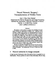
The training inputs of the \two-spirals" problem consists of 194 hx; y i points at which RNi should output 0's or 1's as shown in Fig. 5(a). Each RNi in the SMs has two input, ve hidden units and one output unit. Training of RNi is stopped after 10000 iterations if the total error between the desired and the actual outputs cannot be less than the given value, 0.1. The \two-spirals" problem is learned by a PMSN according to the multi-sieving learning algorithm. After learning, we obtain a PMSN with three R-form sieving modules as shown in Fig. 6(a). The input patterns that are learned by the rst, the second and the third SMs are illustrated in Figs. 5(b) through (d), respectively. The response plots of the PMSN and the rst through the third SMs are illustrated in Figs. 7(a) through (d), respectively. From Figs. 7(b) through (d), it is clear that the \twospirals" problem is decomposed into three relatively manageable subtasks and each subtask is solved by a corresponding sieving module as shown in Fig. 6(a). From Fig. 6(a), we can see that all the sieving modules are processed almost in parallel.

: Freeze all of the parameters of RNm and CNm (if it exists), remove Nvo;m samples which have been successfully classi ed by RNm from Tm , and create a new training set consisting of tm+1 (tm+1 = tm 0 Nvo;m ) samples Tm+1 (TM +1  Tm ), which are not classi ed by RNm .

Step 6

: If CNm exists, construct SMm in the RCform. Otherwise make SMm in R-form.

Step 7

: Join SMm to SMm01 for m > 1 in the parallel structure as shown in Fig. 6.

Step 8

: Select RNm+1 and train it on Tm+1 up to iterations. Let m = m + 1 and go back to Step 2.

Step 9

K

From the above description, we can see that the number of SMs needed for learning a given task is determined by the MSL algorithm automatically. Obviously, there exists a trade-o between the learning capability of RNm and the number of iterations for training RNm .

Modi cation to Trained Network For most of the existing constructive learning networks such as the cascade correlation architecture, even with few simple modi cations to the learning task, all the parameters of the trained network must be re-adjusted. This example illustrates how to implement modi cation to trained PMSNs without de-

Suppose that a PMSN consists of m sieving modules SM1 , SM2, and SMm , the processing time required 1 It should be noted that the control network CN always m learns the classi cation of the valid and the pseudo valid outputs successfully, by assumption

95

1

1

0.8

0.8

0.6

0.6

0.4

0.4

0.2

0.2

0

Input

Valid Output

RN 1 OJU

RN 2 0

0.2

0.4

0.6

0.8

1

0

0.2

(a)

0.4

0.6

0.8

1

OJU

(b)

1

1

0.8

0.8

0.6

0.6

0.4

0.4

0.2

0.2

RN 3 OJU

0

0.2

0.4

(c)

0.6

0.8

1

0

0.2

0.4

0.6

0.8

1

(a)

(d)

Figure 5: The input patterns of the \two-spirals" problem (a), the input patterns classi ed by the rst SM (b), the second SM (c), and the third SM (d), respectively. For black and grey points, the RNm is required to generate output 0 and 1, respectively.

0

Input

Valid Output

RN 1 OJU CN 1

stroying any parameter of the trained recognition networks. In our simulated problem we will try to modify the trained PMSNold , shown in Fig. 6(a), to recognise the updated two-spirals problem (see Fig. 8(a)).

RN 2 OJU CN 2

We present the 16 updated training inputs to RN1 of the PMSNold , we obtain Npvo; 1 = 16 and Nvo; 1 = 0, that is, no updated training input is generalized correctly by RN1 . In a similar way, we obtain Npvo; 2 = 16, Nvo; 2 = 0, Npvo; 3 = 11 and Nvo; 3 = 5. Here Nvo; 3 = 5 means that there are 5 updated training inputs which are generalized properly by RN3 . In order to learn the 16 updated training inputs, three control networks CN1 , CN2 , and CN3 are trained and added to the PMSNold , and the sieving modules in the PMSNold are changed into RCform. The 11 updated training inputs which can not be generalized correctly by RN1 , RN2 and RN3 are learned by a new recognition network RN4 . The modi ed PMSN with four sieving modules, namely PMSNnew , is illustrated in Fig. 6(b). The response plot of PMSNnew is illustrated in Fig. 8(b). Comparing Fig. 7(a) with Fig. 8(b), we can see that the 16 training inputs, which have already been learned by PMSNold , are updated by modifying PMSNold without adjusting the parameters of RN1 , RN2, and RN3 in PMSNold .

RN 3 OJU CN 3

RN 4 OJU

(b) Figure 6: Two PMSNs for learning the \two-spirals" problem (a) and the updated \two-spirals" problem (b), where the control signal to the rst sieving modules is set to \0"

96

1

1

1

0.8

0.8

0.8

0.6

0.6

0.6

0.4

0.4

0.4

0.2

0.2

0.2

0

0 0

0.2

0.4

0.6

0.8

1

0

0.2

(a)

0.4

0.6

0.8

0

1

(b)

1

1

0.8

0.8

0.6

0.6

0.4

0.4

0.2

0.2

0 0.2

0.4

0.6

0.8

1

0.4

(a)

0.6

0.8

1

(b)

Figure 8: The updated two-spirals problem in which 16 training data are dierent from the original twospiral problem (a), and the response plot of the modi ed PMSN (b). [2] Ersory, O. K. and Hong, D. , 1990, \Parallel, selforganizing, hierarchical neural networks", IEEE Trans. on Neural Networks, vol. 1, no.2, pp. 167178.

0 0

0.2

0

(c)

0.2

0.4

0.6

0.8

1

(d)

Figure 7: Response plots of the PMSN (a), the rst SM (b), the second SM (c), and the third SM (d). Black and white represent output of \0" and \1", respectively, and grey represents intermediate value.

[3] Fahlman, S. and Lebiere, C., 1990, \The cascadecorrelation learning architecture", Report CMUCS-90-100, Carnegie-Mellon University. [4] Hechi-Nielsen, R., 1990, \Neurocomputing", Addison-Wesley, Reading, Mass. [5] Lang, K. and Witbrock, M., 1988, \Learning to tell two spirals apart", Proc. of 1988 Connectionist Models Summer School, pp. 52-59, Morgan Kaufmann.

CONCLUSION We have presented a parallel and modular multisieving network architecture for constructive learning. This architecture oers two major advantages over existing constructive learning networks such as the cascade correlation architecture. Firstly, this architecture is a modular structure and the trained modular networks can be modi ed without adjusting all the parameters to learn an updated task. Secondly, all of these modules are connected in parallel. Hence, problems which associate with \deep network" does not exist with this architecture. The response time is almost independent of the number of modules.

[6] Lu, B.-L., Bai, Y., Kita, H. and Nishikawa, Y., 1993, \An ecient multilayer quadratic perceptron for pattern classi cation and function approximation", Proc. of International Joint Conference on Neural Networks, vol. 2, pp. 1385-1388, Nagoya. [7] Lu, B.-L., 1994, \Architectures, learning and inversion algorithms for multilayer neural networks", Ph. D. thesis, Dept. of Electrical Engineering, Kyoto University. [8] Lu, B.-L., Kita, H. and Nishikawa, Y., 1994, \A multi-sieving neural network architecture that decomposes learning tasks automatically", Proceedings of IEEE Conference on Neural Networks, pp. 1319-1324, Orlando, FL.

ACKNOWLEDGEMENT The authors are grateful to Kenneth H. L. Ho for reading the manuscript.

[9] Mezard, M. and Nada, J. P., 1989, \Learning in feedforward layered networks: the tiling algorithm", Journal of Physics A, vol. 22, pp. 2191-2203.

REFERENCES

[10] Rumelhart, D. E., Hinton, G. E. and Williams, R. J., 1986, \Learning representation by backpropagation errors", Nature, vol. 323, pp. 533-536.

[1] Baers, P. T. and Zelle, J. M., 1992, \Growing layers of perceptrons: Introducing the extentron algorithm", Proc. of International Joint Conference on Neural Networks, pp. II-392-II-397, Baltimore, MD.

97