Department of Numerical Analysis and Computer Science TRITA-NA-P0121 • ISSN 1101-2250 • ISRN KTH/NA/P-01/21SE
A Parallel Implementation of a Bayesian Neural Network with Hypercolumns
Christopher Johansson and Anders Lansner
Report from Studies of Artificial Neural Systems (SANS)
Numerical Analysis and Computer Science (Nada) Royal Institute of Technology (KTH) S-100 44 STOCKHOLM, Sweden
A Parallel Implementation of a Bayesian Neural Network with Hypercolumns Christopher Johansson* and Anders Lansner
TRITA-NA-P0121
Abstract A Bayesian Confidence Propagation Neural Network (BCPNN) with hypercolumns is implemented on modern general-purpose parallel computers. Two different parallel programming application program interfaces (APIs) are used, OpenMP and MPI. Hypercolumns is a concept derived from the local connectivity seen between neurons in cortex. The hypercolumns constitute a natural computational grain and enables good parallelism of the BCPNN algorithm. The parallel version of the BCPNN scales well.
Keywords: BCPNN; ANN; Parallel; Hypercolumns; MPI; OpenMP; Neural Network
* E-mail:
[email protected]
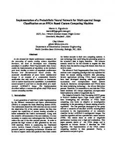
Introduction Executing a sequential implementation of a large Artificial Neural Network (ANN) generally takes a long time and consumes a lot of memory. This makes it difficult to create large ANNs and evaluate complex systems of ANNs, i.e. systems inspired from biology. There is a large amount of natural parallelism incorporated into ANNs. Unfortunately the parallelism in ANNs is different from that of modern and generalpurpose parallel computers. ANNs have a fine grain parallelism while modern computers are more adapted to large grain parallelism. The ANN used is a Bayesian Confidence Propagation Neural Network (BCPNN) with hypercolumns [1, 2]. The BCPNN consists of a number of neurons and these neurons are connected with weighted connections. The connection-weights form a symmetric weight-matrix [3, 4]. Each neuron gets an input from almost all the other neurons in the ANN; this means that the ANN is recurrent [5]. The neurons sum the input from other neurons to determine their own activity. The output from the BCPNN is graded between 0−1. The output is also referred to as the activity of the neurons. The output values are viewed as probabilities [6].
INPUT Hypercolumn 1 Ni (i=1)
Ni (i=2)
j=1 j=2 j=3 j=4 j=5 j=6
Hypercolumn 2 Ni Ni (i=3) (i=4)
Hypercolumn 3 Ni (i=5)
Ni (i=6)
Wij
Wij
Wij
Wij
Wij
Wij
Wij
Wij
Wij
Wij
Wij
Wij
Wij
Wij
Wij
Wij
Wij
Wij
Wij
Wij
Wij
Wij
Wij
Wij
Bi
Bi
Bi
Bi
Bi
Bi
∑
∑
∑
∑
∑
∑
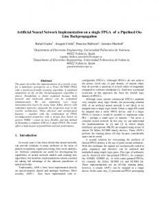
OUTPUT Figure 1 A small recurrent BCPNN with six neurons (Ni) divided into three hypercolumns. A neuron i computes its activity based on the input from the other neurons j and the weights Wij and the bias Bi. Note that there are no recurrent connections within each hypercolumn. Instead, the activation within each hypercolumn is normalized. With some imagination it can be seen how the weights, Wij, form a matrix.
The neurons in the BCPNN are divided into functional groups called hypercolumns [7-10]. A hypercolumn represents an attribute i.e. the colour of an object. The activity of a single neuron in a hypercolumn can be viewed as a probability of that attribute value, i.e. the probability that the object is red. The hypercolumns form a natural way of dealing with the dependences between different values of an attribute. The attributes are assumed to be independent of each other. The activity of the nodes in a hypercolumn sum to one. The BCPNN performs two kinds of operations, learning and retrieval. The network works as an autoassociative memory. During learning the weights are changed based on the presented input. The output of the network is clamped to the input during learning. During retrieval the activity of the neurons change according to the current input and the weight-matrix in an iterative relaxation process. The learning process is incremental. Patterns can be learnt one at a time as opposed to non-incremental learning, where the whole training set (all patterns) must be present when the learning takes place. If the training set is composed of more patterns than can be stored in the network, the network only remembers the latest learnt patterns (provided the learning rate is properly set). A memory that has the ability to forget old patterns in favour of new patterns is called a palimpsest memory [11-13].
The BCPNN with Hypercolumns The continuous time version of the BCPNN update and learning rule is presented in Eq. (1)-(6). Eq. (1)-(4) are used in the training phase, and Eq. (5) and (6) are used in the retrieval phase. The equations were solved with Euler’s forward method. The first letter in a double index, i.e. j, refers to a particular hypercolumn; the second index (primed index) refers to neuron j′ in hypercolumn j. d Λ ii ' (t ) = α ([(1 − λ0 )oii ' (t ) + λ0 ] − Λ ii ' (t )) dt d Λ ii ' jj ' (t ) = α ([(1 − λ02 )oii ' (t )o jj ' (t ) + λ02 ] − Λ ii ' jj ' (t )) dt β ii ' (t ) = log(Λ ii ' (t )) Λ ii ' jj ' (t ) wii ' jj ' (t ) = Λ ii ' (t )Λ jj ' (t ) N Mi dhii ' (t ) = β ii ' (t ) + ∑ log ∑ wii ' jj ' (t )o jj ' (t ) − hii ' (t ) j' dt j
oii ' (t ) =
eGhii ' (t ) ∑ eGhii ' (t )
(1) (2) (3) (4) (5)
(6)
i'
The bias is denoted with ‘β’ in the equations. Patterns of activity are denoted as ‘o’ in the equations. The input to each neuron is denoted as ‘h’ and is called the support value. Connection-weights are denoted as ‘w’.
The equations can be solved with other methods than Euler’s forward method, but since the method is easy to implement and the equations are not stiff, Euler’s forward method is well suited. The use of Euler’s method is also conformant with earlier work done on Bayesian counting neural networks [1]. The input to the BCPNN consists of binary patterns. Only one neuron is active in each hypercolumn of the input patterns. When retrieval is studied, the BCPNN is presented with patterns where the values in 20% of the hypercolumns are randomly changed. A retrieval is classified as correct if the overlap between the input- and output-pattern, after relaxation, is greater than 0.85. The input pattern is denoted as p and the output pattern is denoted as o in Eq. (7).
overlap =
1 H
N
∑o
j
pj
(7)
j =1
A retrieval operation is considered complete when the change of activity between two consecutive steps of the relaxation process is smaller than 10-3·N, where N is the number of neurons. The activity of neuron j in iteration i is defined as oj(i). The change of activity is defined as: N
change of activity = ∑ oij − oij−1
(8)
j =1
The time it takes to train each pattern is fixed. In all experiments both the training and retrieval time was set to 1. Normally the time it takes to retrieve a pattern varies a lot, since the retrieval continues until a stable pattern is found. Here the time-step was set to 0.1, which means that a training-/retrieval-time of 1 corresponds to 10 iterative steps. The storage dynamics and capacity of the BCPNN is mainly controlled by a parameter named alpha, α. The storage dynamics and capacity are also affected by the values of the constant λ0 and the parameter G (gain). The parameter α was set to 0.1 and the parameter G was set to 10 and λ0 was set to 10-4.
Implementation Real neurons communicate via the synapses and generate their output signals simultaneously. Compared with traditional implementations of ANNs, where the output of each neuron is computed sequentially, the neural networks found in nature can be said to run in parallel. If the computations of an ANN are made in parallel a great gain of speed can be achieved. The problem with parallel implementations of ANNs is to update the activity of each neuron through out the entire network. This calls for a high need of communication and as a result makes an efficient parallel implementation difficult.
Parallel Computers
Parallel computer architectures can be divided into two main categories; SIMD (Single Instruction stream, Multiple Data streams) and MIMD (Multiple Instructions streams, Multiple Data streams). The one used here is MIMD and this is also the most common parallel architecture in use today. Previously the BCPNN without hypercolumns have been implemented on computers with the SIMD [14, 15] architecture. Mainly two computers were used, a SGI Onyx 2 (Boye) and an IBM SP (Strindberg). These two computers both have MIMD architecture. Boye has 12 processors and 4 GB of memory. Strindberg is equipped with over 250 processors and has 170 separate processor nodes. Boye uses a memory architecture called shared memory. Shared memory means that all of the processors have access and share the same memory. Strindberg has a memory architecture called distributed memory, which means that each node has its own separate memory. Strindberg has three different types of processors and several different types of nodes. The BCPNN code was always executed on T-nodes. T-nodes have a PPM 2 processor, running at 160 MHz, and are equipped with 256 MB of memory.
Software for Parallel Programming
Two APIs (Application Program Interfaces) were used, the OpenMP API and the MPI API. OpenMP is used on parallel computers with shared memory and the MPI API is used on computers with distributed memory. OpenMP uses threads to split up the computations into separate streams. MPI facilitates the parallel computations with message passing between several concurrently running programs, each program run on a separate node. The terminology differs between shared and distributed memory applications. A crud translation is that a thread corresponds to a node and that a fork or join corresponds to message passing. The work of this report was focused on implementation that used the MPI API. As a consequence much of the text will refer to the terminology and architecture of computers with distributed memory that uses message passing in its applications.
OpenMP
Programming a computer with multiple processors and shared memory difference little from programming a usual single processor computer. An OpenMP [16] program run in one thread until it encounters a part of the program with heavy calculation (that can be executed in parallel) then it splits up into several threads (fork) and performs the calculation. When the particular calculation is finished the execution of the program is continued in a single thread (join). This computational paradigm is called fork-join paradigm.
Programs that use OpenMP are easier to debug than programs that uses MPI. A disadvantage of OpenMP, compared to MPI, is that there is less control over hidden message passing that can degrade performance. OpenMP is mainly introduced into a program through compiler directives (‘#pragma’ remarks in C), but the OpenMP API also contains a few functions. Usually the compiler automatically makes a program parallel, i.e. large loops are split up between the processors, but to ensure compatibility this feature is not standard. The OpenMP API also contains a few library functions. Multiple threads can be run on a processor but usually only one thread is run at a time on each processor. There are several different strategies to how the threads are distributed among the processors. These strategies are concerned with achieving a good load balancing and minimizing the hidden communication between the processors. Usually the standard method is a reasonably good choice. The standard method is that the computational task is split up into several threads. Each processor executes a single thread at a time. When one processor has finished the execution of a thread the execution of a new thread is initiated. This continues until all threads are executed.
MPI
The Message Passing Interface (MPI) was developed in the early 90s [17]. As the name suggest the basic principle is that many programs are run in parallel and communicate with each other via messages to coordinate their computations. Each program runs on a node. A node facilitates a least one processor and memory, therefore a computer with this type of parallel architecture is said to have a distributed memory. When a MPI program executes there are always a constant number of programs, each running on a separate node, running which is a big step from the normal sequential programming paradigm. It is often necessary to rewrite large parts of the program before it can use the MPI API. A MPI program is often hard to debug, especially since it is hard to modularise a MPI program. It is possible to use both OpenMP and MPI on IBM SP computers. IBM SP computers have nodes with more than one processor per node. On each node, with multiple processors, OpenMP can be used. MPI is then used to handle the communication between these nodes. The idea with this concept is that OpenMP is easy to use and a lot of code can be made parallel with OpenMP. MPI is used to a minimum, only to bring it all together. A solution to the communication problem of updating the activity of all neurons in the entire neural network is to allow asynchronous updating between the nodes in the computer. Asynchronous updating cannot be done in the current version of the MPI API. The communication between nodes cannot occur randomly, it has to be determinate, i.e. a program on one node cannot refuse to receive a message, specifically sent to it, from another node. The implication of this is that a least a small message has to be sent that notifies the receiving node if a larger message will be sent or not. The need of asynchronous communication will groove since the parallel computers in the future will have a heterogeneous architecture [18] and the cost of synchronise the computations of a running program will probably increase.
Mapping of the BCPNN onto Hardware
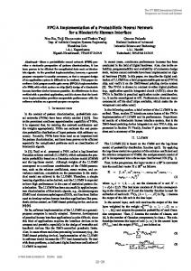
There are many ways the computations of an ANN can be split up, i.e. the computations for each neuron (vector of weights) are distributed or the computations for each weight are distributed. It is also possible to make the parallel computational modules on a higher level, i.e. a system of networks [19] where the computations of each ANN is distributed. If all patterns are present at the beginning of the training phase it is possible to distribute the computations for each pattern. These are just a few ways the computations of a neural network can be distributed [15, 20, 21]. The computations of the BCPNN learning rule are distributed for each hypercolumn (matrix of weights). The computations are distributed on threads in the case of shared memory and on nodes in the case of distributed memory. From an algorithmic point of view it does not matter whether the computations are distributed on nodes or threads and therefore we can collect nodes and threads in the term processing units (PUs). The same way of reasoning can be applied to the operations of message passing and fork-join, which will be called parallel initiations (PIs). Both of these two operations take considerable amounts of time to perform and should be used to a minimum. The neurons in the BCPNN are divided into hypercolumns. The hypercolumn structure allow for a simple mapping of the neurons onto the PUs. The computations of the BCPNN are distributed on several PUs and each PU perform computations on one or more hypercolumns. Dividing the computations between hypercolumns instead of between i.e. the neurons has the advantage of a larger computational grain size. In all experiments, the BCPNN is trained on a set of patterns and then these patterns are retrieved. The training can be preformed on one pattern at a time, but here the training was done in batch mode. Batch mode training means that the whole training set, all patterns, are available at the start of the training and can be copied to each node. This means that only one PI has to be performed during the training phase. The workload of the training phase is easily distributed among the PUs (Figure 2). The iterations of the time-step is done locally in each PU. Only one PI has to be performed for each new pattern. If the training is done in batch mode just one PI has to be performed during the whole training phase and thus allows for extremely large grain parallelism. Learning a pattern requires more floating-point operations (FLOPs) than retrieving a pattern.
Pattern(s) In
The activity is distrubuted to the Nodes
PU 1
PU 2
The weights and bias of hypercolumn 1 are computed. Next time-step
PU 3
The weights and bias of hypercolumn 2 are computed. Next time-step
The weights and bias of hypercolumn 3 are computed. Next time-step
Weight-Matrix and Bias
Figure 2 The training phase of the BCPNN. The network has three hypercolumns and a separate PU handles each. There are no PIs performed between the time-steps, which allows for large grain parallelism. Large grain parallelism and batch mode training makes the training process fast and efficient.
The retrieval phase cannot be implemented with the same large grain parallelism as the training phase. Figure 3 shows the retrieval phase, which facilitates an iterative loop outside of the PUs. For each time-step in the retrieval process the activity of each neuron has to be known to every other neuron. This causes many PIs to occur which means that the need of communication is high. Performing a PI takes a lot of time and this causes the processors to idle. Idle processors results in that the number of floating-point operations per second (FLOPS) is much lower during retrieval than during the training phase. The stop criterion in Figure 3 is not used. Instead the retrieval process is stopped after 10 time-steps.
Activity In (i.e. a distorted pattern)
The activity is distrubuted to the Nodes
PU 1 The activity of hypercolumn 1 is computed.
Next time-step
PU 2 The activity of hypercolumn 2 is computed.
PU 3 The activity of hypercolumn 3 is computed.
A stop criterion is evaluated.
Activity Out
Figure 3 The retrieval phase of the BCPNN. For each time-step a PI has to be performed. This results in bad performance, a low FLOPS value. The stop criterion was not used, instead the retrieval process was stopped after 10 time-steps.
Both the training phase and the retrieval phase are implemented without any computational overhead compared with a single processor implementation. The complexity of both the learning and retrieval operations are Ο(N2) for each pattern. If the number of patterns is increased as the storage capacity of the BCPNN is increased, the complexity becomes Ο(N3.5) for both the learning and the retrieval phase. The BCPNN was implemented in three different versions. One version of the BCPNN code was optimised for a single processor computer. Two other versions of the code were designed to use OpenMP and the MPI API. The MPI version of the code was used with MPICH and run on a regular LAN (Local Area Network). All code was written in C [19] and is available on the Internet [22].
Results Optimisation on a Single Processor
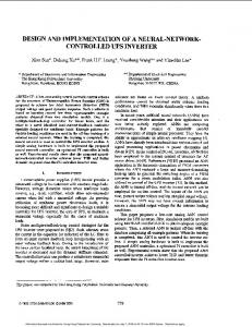
There is a lot to be said about optimisation of computer programs. To start with one should try to get a compiler that supports the hardware and also make sure it is the latest version of the compiler. It is also important to use the compiler option -Ox (x=1-3), which means that the compiler will use optimisation. The option O3 must be used with care, since it can alter the function of the code. Choosing the right type for the variables is also important. I use binary patterns in my program. These patterns were at first represented with the type char (one byte), but are now represented with short int (two bytes). I changed the type because the processor has to convert the char into an int before it can perform operations upon it. The weight-matrix was at first stored as double, but to save memory the type was changed to float. Memory access should be done locally i.e. it is faster to access elements j and j+1 than it is to access elements j and j+100. The element j+1 will be found in the cache memory and there will be no need to access the main memory. The benefit of local access arises from the fact that when data is read from memory it is done in big chunks (memory blocks) and these memory blocks are placed in the fast cache memory. It is also important to try to avoid branches (i.e. if statements), especially in loops. Branches disable the use of the pipeline (the pipeline allows the processor to execute several instructions simultaneously). A good rule of thumb is that if the code looks “clean” it often is good. Figure 2 shows the performance of five different processors on four different computers. The BCPNN program, a network consisting of 256 neurons that was trained with 600 patterns, was compiled with different compilers, GCC 3.0 was used on the PC, a SUN compiler was used on Boye (SGI Onyx 2) and an IBM compiler was used on Strindberg (IBM SP). The speed of the training process depends heavily on the “number crunching” capability of the computer. The speed of the retrieval process depends on the memory bandwidth. Boye executes the retrieval very quickly since it has a high memory bandwidth compared to the other computers. The code was compiled with different compilers on each computer. The compiler option O3 was used with all compilers.
Training
Retrieval
45 40 35 30 Time (s)
25 20 15 10 5 0 160 MHz
222 MHz
500 MHz
195 MHz
PPM 2
PPM 3
Intel PIII
SGI R10000
IBM SP
IBM SP
PC
SGI Onyx2
Figure 4 A comparison of four processors used on three different computers running a network with 256 neurons and a training set of 600 patterns. The training phase is a good measure of the processors number crunching capability and the retrieval phase can be used to give a hint on the computers memory bandwidth.
Scaling on Multiple Processors
The scalability of the parallel implementations, the implementations on Boye and Strindberg, of the BCPNN were tested in several ways. The configurations, in terms of used processors, between the runs on Boye and Strindberg differs a little. One reason is that Strindberg has more processors than Boye. Another reason is that the number of hypercolumns does not have to be an integer multiple of the number of processors when the OpenMP implementation is used. To enable the interpretation of Figure 5 and Figure 6 the equations (9)-(11) are defined. Tsingle is the time required to execute a program optimised for a single processor computer. NP is the number of processors. Linear speed-up is then defined as the speed-up you get if every added processor would work at 100% efficiency. Linear SpeedUp =
Tsingle
(9)
( NP ⋅ T ) single
Relative speed-up is defined as how much faster a program, optimised for a multiple processor computer, gets for each new processor that is used. Tmultiple is the time required to execute the program. Relative SpeedUp =
Tmultiple
( NP ⋅ T
multiple
)
(10)
Absolute speed-up is the improvement you get from the parallel version of the program compared with the program optimised for a single processor.
Absolute SpeedUp =
Tmultiple
( NP ⋅ T )
(11)
single
There are occasions when the parallel implementation of a program runs faster than expected, i.e. the speed-up is larger than the linear speed-up. This phenomenon is called hyper linear speed-up. Hyper linear speed-up can occur for several reasons i.e. better cache usage because the data fits entirely into the cache. The relative speed-up is a good measure of how well the parallel code scales. But the relative speed-up does not indicate how good the parallel implementation is i.e. if there are large computational overheads in the parallel code. The actual performance of the parallel implementation can be evaluated with the absolute speed-up. The measurements of speed-up, defined in Eq. (9)-(11), are applied on data from both the OpenMP (Figure 5) and the MPI (Figure 6) adapted version of the BCPNN code. The BCPNN consisted of 400 neurons and was trained with 1200 patterns. A BCPNN consisting of 400 neurons and using its palimpsest properties can store about 400 patterns [23]. The relative speed-up of the training phase is nearly linear (Figure 5A, Figure 6A), which is very good. The absolute speed-up is less than half of the relative speed-up in both Figure 5A and Figure 6A. The low absolute speed-up is caused by the slow execution of the parallel version of the BCPNN training phase code. Cache misses is probably a large cause of the slow execution of the parallel implementation. The parallel implementation of the BCPNN code has a divided connection matrix and as a consequence large loops are divided into smaller loops. This probably cause cache misses to occur. In the end the parallel, reorganized, code of the training phase is more than twice as slow as the single processor code. The parallel version of the training phase code scales well but it is slower than the code adapted for a single processor. The relative speed-up of the retrieval phase is not linear (Figure 5B, Figure 6B). The absolute speed-up is almost has high as the relative speed-up. The parallel implementation of the BCPNN retrieval phase code is almost as fast as the code used for a single processor. The implementation of the parallel code of the retrieval phase is almost as fast as the code adapted for a single processor but it does not scale as well as the parallel code used for the training phase. Both the relative and absolute speed-up of the OpenMP and MPI adapted versions of the BCPNN code have the same characteristics up to 10 processors. When the number of processors is increased to 20, using the MPI version of the retrieval phase code, the expected corresponding speed-up is abundant. The combined execution time of both the training and retrieval phase, of a BCPNN consisting of 400 neurons and trained with 1200 patterns, was compared between Strindberg and Boye (Figure 7). Strindberg has the ability to use more processors and is thus faster than Boye. If both Boye and Strindberg use the same number of processors then Boye is faster.
Learning Linear Speed-Up
Relative Speed-Up
Absolute Speed-Up
10 9 8 Speed-Up
7 6 5 4 3 2 1 0 1
2
3
4
5
6
7
8
9
10
Processors
A Retrieval Linear Speed-Up
Relative Speed-Up
Absolute Speed-Up
10 9 8 Speed-Up
7 6 5 4 3 2 1 0 1
2
3
4
5
6
7
8
9
10
Processors
B Figure 5 The speed-up on Boye with the OpenMP adapted version of the code. (A) The speed-up of the training phase. (B) The speed-up of the retrieval phase.
The parallel implementation on Strindberg is faster then the implementation optimised for a single processor when two or more processors are used. The parallel implementation on Boye has to be run on three or more processors to execute faster then the single processor implementation (Figure 7). Figure 8 shows the execution time plotted against the size of the network. The network was trained with 50 patterns. Two series of simulations were made. In the first series the BCPNN was run on 10 nodes and in the second series the BCPNN was run on H nodes, where H equals the number of hypercolumns and is defined as H= N e u r o n s . As the network becomes larger, the number of hypercolumns increases as the square of the total number of neurons and thus H is increased i.e. if a network consists of 104 neurons H is 100. The retrieval time increases more steeply when the network size is increased beyond 1000 neurons. Since this increase is present for both of the simulated series, it cannot be an artefact of the transmission buffer. Strindberg’s transmission buffer allows MPI calls to be buffered if the number of concurrent tasks (used nodes) is small. Cache misses probably cause the deviation of the retrieval time (Figure 8).
Linear Speed-Up
Relative Speed-Up
Absolute Speed-Up
20 18 16
Speed-Up
14 12 10 8 6 4 2 0 1
2
3
4
5
6
7
8
9
10 11 12 13 14 15 16 17 18 19 20 Processors
A Linear Speed-Up
Relative Speed-Up
Absolute Speed-Up
20 18 16
Speed-Up
14 12 10 8 6 4 2 0 1
2
3
4
5
6
7
8
9
10 11 12 13 14 15 16 17 18 19 20 Processors
B Figure 6 The speed-up on Strindberg with the OpenMP adapted version of the code. (A) The speed-up of the training phase. (B) The speed-up of the retrieval phase.
When H nodes were used the execution time only increased as k1·N1.5 where N is the number of neurons. In the case where there were a constant number of nodes the execution time increased as k2·N2. The factor k1 was about ten times larger than k2. The execution time, of a network with 104 neurons, was considerably decreased, almost a factor 10, when H=100 nodes where used instead of 10 nodes (Figure 8). The performance of neural network computations is sometimes measured in connection updates per second (CUPS) and connections per second (CPS) [24]. The number of altered connection per second during the training phase is measured in CUPS and the number of read connections during the retrieval phase is measured in CPS. The performance of the parallel implementation of the BCPNN run on 100 nodes is CUPS≈140·106 and CPS≈42·106.
Execution Time, Execution Time, Execution Time, Execution Time,
Boye Strindberg Single Processor, Boye Single Processor, Strindberg
2
Time (s)
10
1
10
2
4
6
8
10 12 Processors
14
16
18
20
Figure 7 The execution time on Boye and Strindberg. The OpenMP adapted code was run on Boye and the MPI adapted code was run on Strindberg. The execution time of the code optimised for a single processor is plotted as horizontal lines.
3
10
Training, Retrieval, Training, Retrieval,
10 Nodes 10 Nodes H Nodes H Nodes
2
Time (s)
10
1
10
0
10
3
4
10
10 Neurons
Figure 8 The execution time on Strindberg. The solid line represents the execution time on 10 nodes and the dotted line represents the execution time on H nodes, where H is the number of hypercolumns. The BCPNN was used with 50 patterns.
Alternative Platforms
MPICH is a freely available, portable implementation of MPI. MPICH can be run on a LAN (Local Area Network). There are implementations of MPICH for a large number of computers. The MPI version of the program was run on ten SUN Blade 100 computers connected with a 100 Mbps Ethernet network. The BCPNN consisted of 400 neurons and was trained with 1200 patterns. The large limitation of using computers connected with a standard 100 Mbps Ethernet is that the communication between computers takes a lot of time. This fact is clearly visible in Figure 9. The time it takes to train the network is comparable between the three computers, but the retrieval phase is much slower on the LAN / MPICH constellation. Ten processors were used on all computers, considering the LAN as a single computer. Load balancing can be a problem when using MPICH. One or more of the computers in the LAN can be shared with other users or the network can be heavily loaded, which will degrade the performance. MPICH is, however, a very neat way of building a cheap parallel computer. Training
Retrieval
200 180 160
Time (s)
140 120 100 80 60 40 20 0
Boye
Strindberg
LAN
Figure 9 A comparison between Boye, Strindberg and a LAN composed of SUN Blade 100 computers connected with a 100Mbit Ethernet. 10 nodes were used in each of the three cases. Boye run the OpenMP version of the program, while Strindberg and the LAN run the MPI version.
Extensions of the MPI Implementation
The goal of the optimisation was to speed-up the communication between nodes during retrieval. To achieve this we made the activity binary after each step of relaxation, Eq. (6) was changed to Eq. (12). 1 if i ' = arg max{hik (t )} k Oii ' (t ) = 0 else
(12)
Replacing Eq. (6) with Eq. (12) changes the amount of computations only with a small constant factor. The storage capacity of the binary output version of the BCPNN matches that of the regular BCPNN with continuous valued output (Figure 10). The binary output from each hypercolumn, containing n neurons, makes it possible to shrink the message size from n floats to a single int. But the number of messages is not decreased. Experiments showed that a smaller size of the messages did not improve performance. If the only task is pattern association the weights as well as the activity of the BCPNN can be reduced to a binary representations. If this is done the BCPNN is reduced to a Willshav network [3]. When a large number of patterns is stored in the BCPNN the weights tend to be distributed in a binary fashion, half of the weights are excitatory and the other half of the weights are inhibitory [19]. A conclusion of this discussion is that if the field of usage is known, large optimisations can be done [25]. The MPI API contains something called non-blocking calls. When a non-blocking call is initiated the processor does not have to wait for that call to return, instead the execution can continue while the communication is performed. The MPI version of the BCPNN code was rewritten with non-blocking calls but it did not result in a performance improvement. The conclusion is that the BCPNN code cannot utilize the benefits of non-blocking calls since there are no instructions that can be executed in the processor time made available by the non-blocking calls.
1 Continuous Output Binary Output
0.9 0.8
Retrieval Ratio
0.7 0.6 0.5 0.4 0.3 0.2 0.1 0
0
20
40
60
80
100 120 Patterns
140
160
180
200
Figure 10 The plot shows the fraction of retrieved patterns that are classified as correctly retrieved. Pattern 200 is the most recently learned pattern. The implementation of the BCPNN, with binary activity, is compared with the regular implementation of the BCPNN, with continuous valued activities.
Analysis of the Implementation The computational resources needed to run a BCPNN was analysed. This analysis is used to identify the hardware requirements and the bottlenecks of the computations.
It is difficult to determine how many FLOPs mathematical functions such as log() and exp() use, especially since it differs much on different computers. From results using a monitoring program, ssrun, on Boye the number of FLOPs used by these functions were estimated; Log()∼13 FLOP and Exp()∼20 FLOP. The memory and computational resources used by the BCPNN code were estimated by studying the code. These calculations are not exact, but give a good approximation. The amount of transferred data includes both the data transferred during the training and the retrieval phase. The memory requirements and the amount of transferred data are measured in bytes. Eq. (13)-(18) were used to construct Table 1. The variables are stored as 4 bytes floats. Memory = N 2 + N·P + 4·N + 2·P
(13)
2
2
FLOPtraining = 2·N + N·Log() + (60·N + 50·N)·P
(14)
FLOPretrieval = (Tretrieval ·(3·N 2 + (Log()+2)·H·N + (Exp()+10)·N) + N·2)·P Messages training = (D-1)·P
(15) (16)
Messages retrieval = ((D-1)·4)·P
(17)
Data Transferred = (3·(D-1)·N+H 2 +(D-1))·P
(18)
P = Number of Patterns N = Total number of Neurons H = N =Number of Hypercolumns D = Number of Nodes Tretrieval = 10 = Number of relaxation steps
Real Neurons
Mini Columns
Hyper Columns
Memory (kB)
Training (FLOP)
Retrieval (FLOP)
Total (FLOP)
Data Messages Trans. (kB)
1,0E+04
1,0E+02
10
1,6E+02
6,3E+05
4,8E+05
1,1E+06
45
9,0E+01
1,0E+06
1,0E+04
100
1,6E+06
6,2E+09
3,2E+09
9,4E+09
495
9,7E+03
“mouse”
1,0E+08
1,0E+06
1000
1,6E+10
6,2E+13
3,0E+13
9,2E+13
4995
9,8E+06
“human”
1,0E+10
1,0E+08
10000
1,6E+14
6,2E+17
3,0E+17
9,2E+17
49995
9,8E+09
Table 1 The table gives an approximation on the computational resources needed for running large BCPNN. The total number of calculations can be seen as an upper limit (all patterns do not need to be retrieved). All numbers were calculated to be stored as 4 byte floats.
Based on Eq. (13)-(18) we estimated the computational resources needed to implement neural networks of the size found in nature. Every artificial neuron is thought to represent a mini-column. The size of a mini-column is in the order of 102 neurons [8]. A hypercolumn is thought to be composed of about 103 mini-columns. In Table 1 the values computed for the entry ‘human’ were based on a network that consisted of 104 hypercolumns. Table 1 only provides coarse approximations of what can be done with more neurons and the numbers should not be taken too seriously, i.e. the networks are fully recurrent while biological neural networks are sparsely connected.
Discussion If large networks are to be simulated it is important to use the parallel nature of the neural computations. The natural, small grain, parallelism in ANNs is not well suited to be mapped onto modern general-purpose parallel computers. In an attempt to make the computational grains large we exploited the hypercolumns structure in the BCPNN. The BCPNN with hypercolumns was implemented with two different APIs, OpenMP and MPI. The parallel BCPNN code was tested on several computers. It was shown that the computations of the BCPNN scaled well. The BCPNN was run on up to 100 processors. The training phase scaled almost linearly. The retrieval phase scaled relatively good but not as good as the training phase. OpenMP is a good alternative for medium sized BCPNNs. When the BCPNN is big and there is a need for a large number of processors to run the application the only alternative is to use MPI. It is possible to use both OpenMP and MPI on IBM SP computers. In the future it will probably be common to use multiple types of APIs on heterogeneous computers. A number of optimisation ideas were tested, but none of them proved to be useful. It would be interesting to use asynchronous communication. Asynchronous communication cannot be implemented with MPI, at least a small message has to be sent to inform the receiver whether a message will be sent or not. When the BCPNN uses binary output the message size becomes much smaller but the number of messages is not decreased and hence the performance is not improved. All BCPNN used fully recurrent connections but it would be interesting to use sparse connection. There are similar problems arising in both parallel and hardware implementations i.e. the need of an effective implementation of the communication between the hypercolumns. A continuation of the work in this report is to study how the communication can be implemented more effectively and also make a thorough analysis of the implications and requirements on the communication. The ultimate step in the pursuit of parallelism is to implement the BCPNN in hardware, i.e. on a FPGA chip.
References 1. 2. 3. 4. 5. 6. 7.
8.
9. 10.
11. 12. 13. 14.
15.
16. 17. 18. 19. 20. 21. 22. 23. 24.
25.
Lansner, A. and Ö. Ekeberg, A one-layer feedback artificial neural network with a Bayesian learning rule. Int. J. Neural Systems, 1989. 1: p. 77-87. Sandberg, A., et al., Bayesian attractor networks with incremental learning. Network: Computation in neural systems, 2000. Hertz, J., A. Krogh, and R.G. Palmer, Introduction to the Theory of Neural Computation. 1991: Addison-Wesely. Hopfield, J.J., Neural networks and physical systems with emergent collective computational abilities. Proc Natl Acad Sci USA, 1982. 79(8): p. 2554-8. Lansner, A. A recurrent bayesian ANN capable of extracting prototypes from unlabeled and noisy examples. in Artificial Neural Networks. 1991. Espoo, Finland: Elsevier, Amsterdam. Holst, A., The Use of a Bayesian Neural Network Model for Classification Tasks, in Dept. of Numerical Analysis and Computing Science. 1997, Kungl. Tekniska Högskolan, Stockholm. Kandel, E.R., J.H. Schwartz, and T.M. Jessell, The Anatomical Organization of the CNS, Coding of Sensory Information, in Principles of Neural Science. 2000, McGraw-Hill Companies. p. 318-336, 411-429. Fransén, E. and A. Lansner, A model of cortical associative memory based on a horizontal network of connected columns. Network: Computation in Neural Systems, 1998. 9: p. 235264. Calvin, W.H., Cortical Columns, Modules, and Hebbian Cell Assemblies, in The handbook of brain theory and neural networks. 1995, Bradford Books / MIT Press. p. 269-272. Holst, A. and A. Lansner, A Higher Order Bayesian Neural Network for Classification and Diagnosis, in Applied Decision Technologies: Computational Learning and Probabilistic Reasoning, A. Gammerman, Editor. 1996, John Wiley & Sons Ltd.: New York. p. 251-260. Parisi, G., A memory which forgets. J. Phys., 1986. 19: p. 617-620. Sandberg, A., et al., A Palimpsest Memory based on an Incremental Bayesian Learning Rule. Neurocomputing, 1999. 32-33: p. 987-994. Nadal, J.P., et al., Networks of formal neurons and memory palimpsests. Europhysics Letter, 1986. 1(10): p. 535-542. Hammarlund, P., Techniques for Efficient Parallel Scientific Computing. 1996, Royal Institute of Technology, Stockholm, Sweden, Dept. of Numerical Analysis and Computing Science. Levin, B., On Extensions, Parallel Implementation and Applications of a Bayesian Neural Network. 1995, Royal Institute of Technology, Stockholm, Sweden, Dept. of Numerical Analysis and Computing Science. OpenMP C and C++ Application Program Interface. 1998, OpenMP Architecture Review Board. MPI: A Message-Passing Interface Standard. 1995, University of Tennessee, Knoxville, Tennessee. Mahinthakumar, G., et al. Multivariate Geographic Clustering in a Metacomputing Environment Using Globus. in ACM/IEEE SC99 Conference. 1999. Portland, OR. Johansson, C., A Study of Interacting Bayesian Recurrent Neural Networks with Incremental Learning, in NADA. 2001, KTH: Stockholm. p. 71. Misra, M., Parallel Environments for Implementing Neural Networks. Neural Computing Surveys, 1997: p. 48-60. Vialle, S., Y. Lallement, and T. Cornu., Design and implementation of a parallel cellular language for MIMD architectures. Computer languages, 1998. Johansson, C., C-Code (Parallel BCPNN). 2001. Johansson, C., A Capacity Study of a Bayesian Neural Network with Hypercolumns. 2001, Nada, SANS: Stockholm. Sundararajan, N., P. Saratchandran, and J. Torresen, Introduction. Chapter 1, in Parallel Architectures for Artificial Neural Networks, N. Sundararajan and P. Saratchandran, Editors. 1998, IEEE CS Press. p. 1-40. Ruckert, U. and U. Witkowski. Silicon Artificial Neural Networks. in International Conference on Artificial Neural Networks. 1998. Skövde, Sweden: Springer.