IBM Data Explorer is a data-flow based visualization system providing numerous visualization and analysis algorithms for its users. The DX software architecture ...
Los Alamos National Laboratory – Technical Report #LAUR-00-1620
A Parallel Approach for Efficiently Visualizing Extremely Large, Time-Varying Datasets James Ahrens Los Alamos National Laboratory
Charles Law, Will Schroeder, Ken Martin Kitware Inc.
Abstract
executes in parallel on different data elements) to achieve improved performance on a long time series.
A significant unsolved problem in scientific visualization is how to efficiently visualize extremely large time-varying datasets. Using parallelism provides a promising solution. One drawback of this approach is the high overhead and specialized knowledge often required to create parallel visualization programs. In this paper, we present a parallel visualization system that is scalable, portable and encapsulates parallel programming details for its users. Our approach was to augment an existing visualization system, the visualization toolkit(VTK). Process and communication abstractions were added in order to support task, pipeline and data parallelism. The resulting system allows users to quickly write parallel visualization programs and avoid rewriting these programs when porting to new platforms. The performance of a collection of parallel visualization programs written using this system and run on both a cluster of SGI Origin 2000s and a Linux-based PC cluster is presented. In addition to showing the utility of our approach, the results offer a comparison of the performance of commodity-based computing clusters.
�
Keywords: parallel, distributed, visualization, large data
�
1 Introduction Scientists are using computer simulations to resolve models of real world phenomenon, including models of the earth’s climate and oceans and accelerator physics dynamics. With additional computing power and algorithmic advances, these models have been resolved to more detailed levels of resolution, increasing our understanding of the world around us. Key to this process is the visualization and analysis of simulation results. Simulations are usually run in parallel on clusters of high-bandwidth supercomputers, such as SGI’s Origin 2000 series or clusters of PCs. The resulting datasets are so massive in size they require the use of parallel computing resources of similar magnitude in order to effectively visualize them. On a smaller scale, single desktop PCs are now available with multiple CPUs. As both large and small scale parallel computing resources become commonplace for scientists, so must a parallel visualization software system that effectively utilize these resources. A useful starting point for creating a parallel visualization system to support these needs is to build upon an existing visualization system, the visualization toolkit(VTK)[16]. The toolkit contains many serial visualization, graphics and imaging algorithms and is portable to a variety of hardware platforms and operating systems. We had a number of goals for this system:
�
Scalability - Scalability is the ability of a system to use increasing numbers of computing resources to more efficiently process large datasets. The system should support data parallelism (i.e. when a large dataset is partitioned into independent subsets that are processed in parallel) to achieve scalable performance on datasets of massive size. It also should support pipeline parallelism (i.e. when a sequence of algorithms
Michael Papka Argonne National Laboratory
�
Portability - Portability is critical to users with access to heterogeneous platforms since platform availability can change due to crashes, maintenance, purchases and removal. If the user’s visualization system is portable then they can flexibly choose the best available platform instead of being constrained only to the availability of a specific platform. The system should be portable between platforms with different operating systems and underlying hardware, including between shared and distributed-memory multiprocessors. Full functionality - The system should support most of the functionality of VTK, offering parallel versions of the algorithms available. Supporting a full range of parallel visualization algorithms is critical to effectively processing large datasets since the alternative, interspersing serial algorithms with parallel algorithms can significantly degrade performance. Abstraction of complexity for users and developers - Writing correct and efficient parallel programs is difficult for users. The system should encapsulate parallel computing details in order to simplify the creation of parallel visualization programs.
The next section describe related work in parallel visualization algorithms and systems. It characterizes the three possible types of parallelism available in parallel visualization systems: task, pipeline and data parallelism. This paper contributes a design and implementation for a parallel visualization system that supports these types of parallelism on shared and distributed memory processors. The next section describes the fundamental abstractions neccessary to support parallelism (i.e. process and communication objects) and a design for these objects that support demand-driven data-flow execution semantics. Then we describe the addition of each type of parallelism and present performance results for a parallel visualization application that uses each type.
2 Related Work Previous approaches to visualizing large datasets using parallelism include parallel visualization algorithms and systems. Much of the previous algorithmic work in the field of parallel visualization has focus on the area of parallel rendering. Parallel rendering approaches include photo-realistic rendering (i.e. ray tracing, radiosity and particle tracing)[15], polygon rendering[2] and volume rendering[18, 17]. Additional work has focused on parallel isourfacing[6, 13] and geometry optimization[7]. These efforts are complimentary to the our efforts since our goal is the creation of a fully functional visualization system. Previous algorithmic work can be integrated into the toolkit as modules further augmenting the toolkit’s functionality for users.
Los Alamos National Laboratory – Technical Report #LAUR-00-1620
A
memory task parallelism[12]. SCIRun also uses a centralized executive and in this way is similar to Data Explorer. AVS is another popular data-flow visualization system that provides a similar parallel architecture and support. A prototype extension supported data parallelism on the CM-5[9]. A speculation as to why these systems evolved with a centralized executive is they all provide a tightly integrated programming environment that supports the interactive construction, execution and debugging of programs via a graphical user interface. The existence of a single point of control for program construction and execution (i.e. the GUI) may have lead to the creation of a related centralized executive. Designing an efficient mechanism for controlling large number of processes from a single centralized executive is difficult. In contrast to these systems, the parallel visualization system described in this paper avoids the use of a centralized executive and therefore provides a more scalable solution. A distinguishing feature of our system is its seamless support for task, data and pipeline parallelism on both distributed and shared memory multiprocessors.
B
C
D
Figure 1: A sample data flow graph
Other related parallel data-flow based visualization systems include IBM Data Explorer(DX)[4, 1], AVS Express[5] and SCIRun[14]. In these data-flow based visualization systems we refer to a unit of execution as a module. Each module has a set of inputs and outputs. Module inputs and outputs can be interconnected so that the output of one module is passed as an input to another module. In a data-flow based visualization system there are three fundamental types of parallelism. The first type of parallelism is task parallelism[3]. This type of parallelism occurs when independent modules in the data-flow graph execute in parallel. Figure 1 shows a data-flow program graph. The ovals denote modules and the connecting lines denote output and input connections between the modules. Task parallelism occurs in the graph shown in Figure 1, when module A and B execute in parallel. The second type of parallelism is pipeline parallelism. This type of parallelism occurs when a series of connected modules execute in parallel on independent data elements. These elements are usually elements of a time series or independent subsets of a single dataset. Pipeline parallelism occurs in the graph shown in Figure 1, if module A, C and D execute in parallel. The third type of parallelism is data parallelism. This is when a module itself executes in parallel. Data parallelism occurs in Figure 1, if module A executes in parallel, for example, if it reads data in parallel. Each type of parallelism is useful in different situations. Task parallelism is useful for running program graphs with many independent branches, such as those that implement parameter studies, in parallel. Pipeline parallelism is useful for processing timevarying datasets with many independent resources, for example, simultaneously reading from disk, computing results and rendering with graphics hardware. Data parallelism is useful for processing large datasets. System models for achieving parallelism including shared-memory and distributed-memory processes. IBM Data Explorer is a data-flow based visualization system providing numerous visualization and analysis algorithms for its users. The DX software architecture relies on a centralized executive to instantiate, allocate memory and execute modules. DX supports threaded data-parallelism on shared-memory multiprocessors and distributed task parallelism. Both mechanisms were designed to support parallelism in the context of a centralized executive. For example, task parallelism is achieved by a remote module that informs the executive it is ready to execute and waits for a signal from the executive before continuing. SCIRun is a data flow based simulation and visualization system that supports interactive computational steering. SCIRun provides threaded task and data parallelism on shared-memory multiprocessors[8]. An extension to SCIRun permits distributed-
3 Supporting multiple processes In data-flow based visualization systems, visualization programs are constructed by instantiating modules and connecting their inputs and outputs together to form a data-flow program graph. Once created, a program graph is placed in a persistent update state. In this state, when an update request is made, modules in the program automatically execute if their input data is out of date. Automatic updates let users avoid writing program specific update routines, such as, specific system code for automatically loading the elements of a time series or code for deciding which modules to execute after a program parameter change. Implementing automatic program updates requires the support of a number of additional services:
� � �
the ability to share data between modules the ability to run a program persistently the ability to execute module methods
Most of these services are trivial to provide for serial programs but are a challenge to provide for parallel programs. This section describes how these services are implemented with multiple processes and how the implementation achieves our goals of portability and abstraction of complexity. Our approach to designing and building our parallel visualization system was to augment VTK. To support parallelism, the first step was to add a system process object1 . The object abstracts whether the system process is a distributed (via MPI) or shared-memory process (via pthreads or sprocs2 ). The programmer can select the process type at run-time when the process is instantiated.
3.1 Sharing data between modules Data sharing between modules is required to implement data-flow semantics. In a serial program, data sharing is achieved via a language mechanism such as a pointer or a direct reference. The parallel visualization system described in this paper is written in C++, as is VTK. Data sharing between modules that reside in different 1 This should not be confused with the process object currently in VTK. The system process object that is being added provides an abstraction of a unit of execution. The existing process object in VTK is a data processing object. 2 A SGI-specific shared-memory process library.
2
Los Alamos National Laboratory – Technical Report #LAUR-00-1620 0 void module::Update() { 1 2 For each input { 3 this->input->Update(); 4 calculate latest_input_modified_time; 5 } 6 7 if (this->modified_time < 8 latest_input_modified_time) then { 9 this->Execute(); 10 this->modified_time = 11 get_latest_modified_time(); 12 } 13 }
processes is not directly supported in C++. Therefore communication methods were added to the system process object to support data sharing between modules in different processes. These methods implement data sends and receives between processes of all VTK data structures. For efficiency, two different implementations, one for communicating between distributed-memory processes and one for communicating between shared-memory processes were created. Encapsulating the communication methods in the system process object supports program portability between shared and distributed-memory multiprocessors. Two issues must be addressed in the implementation of the communication methods: process synchronization and data sharing. With distributed-memory processes, synchronization is achieved by using an underlying message passing package, in the current implementation, MPI. Data structures must be converted to a contiguous memory representation in order to be passed as messages between processes. There are a number of different data structures that are part of VTK’s data model including data structures for structured points and grids, unstructured grids and graphic elements. A contiguous representation is created when these structures are written to and read from a file. In VTK, file streams from the C++ iostream library are used to perform file I/O. The iostream library also supports string streams. All data structure reader and writer objects were extended to read and write strings in a binary format in addition to files. In the sending process, the VTK object to be sent is written to a string, the string is then sent as a message to the receiving process. In the receiving process, the message is received and a VTK object is instantiated by reading from the string. With shared-memory processes, synchronization is achieved by a locking mechanism that forces the sending process to wait until its message is received. Data sharing is achieved by making a shallow copy of the shared data object.
Figure 2: Pseudocode for Module Update Method
3.4 Automatic program update via demand driven data-flow semantics The parallel visualization system supports the demand-driven dataflow execution semantics of VTK. These semantics are implemented as follows: each module contains a update method and an execute method. When run, a module’s update method requests the update of each of its inputs to ensure that they are up to date. These in turn make recursive calls to ensure their inputs are up to date. Once the update calls return indicating its inputs are up to date, a test is made to see if the module’s execute method needs to be called. The module’s execute method is called if its inputs have been modified. The system tracks modified times via a timestamp mechanism. Figure 2 presents a pseudocode listing of the update mechanism. In a serial program, implementing the update method described above is straightforward. In a parallel program, a number of issues arise:
3.2 Program persistence
�
In a serial program, program persistence is usually implemented via the program’s interactive event loop. The event loop is started as the last statement of the program. It continuously waits for user events (such as mouse and keyboard presses) and responds with pre-defined functions. In a parallel program, most processes do not contain an interaction driven event loop. Instead, a wait method was added to the system process object. The last executable statement in each process calls this method. The wait method contains code to receive messages, respond to remote method invocations and update requests from other processes. The method does not exit until receiving a completion message. With this method, parallel programs can be placed in a persistent state. This solution is scalable, since each process asynchronously responses to incoming requests without coordination with a centralized controller.
� �
3.3 Executing module methods Another useful service is the ability to modify module parameters of an executing program. For example, the user may wish to interactively change an isosurface value. In a serial program, this is accomplished by invoking a module method. In a parallel program, modifying module parameters is more complex because modules reside in different processes. Therefore the system process object, also provides a remote method invocation service. Each process registers module methods that can be invoked by a remote process. These methods are assigned unique tags. When a program is in a persistent state, a remote process with these tags can invoke these methods.
Propagating updates – In a parallel program, update requests need to propagate between modules that reside in different processes. Thus, the remote invocation service is used to handle these requests. Propagating module outputs – In a parallel program, modules in different processes share input/output data. Thus the communication methods are used to provide data sharing across process boundaries. Modified times – Modified times are tracked via a global counter in each process. Thus, comparing timestamps from different processes is meaningless. To address this issue, the parallel update protocol sends a local timestamp (from the updating process to the requesting process) when an input is updated. This timestamp is stored by the requesting process and sent back to the updating process when the next update occurs. Since the timestamp originated in the updating process, it is a valid timestamp and can be used to test whether the requesting process’s input is up to date.
The ability to connect modules across process boundaries is implemented as a port object. When a user wants to connect modules that reside in different processes they connect an output port module as the last module of the first process and then connect an input port module as the first module of the second process. Port objects encapsulate the services need to support demand driven updates between processes. In the future, a port object will be used for all
3
Los Alamos National Laboratory – Technical Report #LAUR-00-1620 module connections and incorporated into the module object definition. Thus, users will no longer need to explicitly create port objects. In summary, process and port objects allow users to write portable visualization program graphs that execute in multiple processes. Additional functionality needs to be added to exploit task, data and pipeline parallelism.
ReadVectors1
ReadSalinity
4 Supporting parallelism This section describes how support for task, pipeline and data parallelism was added. For each type of parallelism, a visualization application is presented. These applications visualize the results of ocean and galactic dynamics simulations. The applications are run on the nodes of an SGI Origin 2000 cluster and a PC cluster. The Origin cluster contains 16 128-way shared-memory multiprocessors. The processors are MIPS R10000s running at 250 Mhz. Note these processors can issue two instructions per cycle. Each multiprocessor runs Irix 6.5, has 32 GBs of shared memory, and is connected via a HIPPI network to other nodes in the cluster. The PC cluster contains 128 dual processor personal computers. Each proccesor is a Pentium III running at 500 Mhz. Each PC runs Linux, has 1 GB of memory and is connected via a Myrinet network to the other nodes in the cluster.
ReadTemp
Shrink
GeometryFilter
IsoSurface
ClipPolyData
Decimate
ExtractZComponent
Threshold1
Mask1
Glyph1
ReadVectors2
ReadVectors3
Divergence
Magnitude
Threshold2
StreamLines
Mask2
ElevationScalars
Render
Figure 3: Task parallelism graph The parallel implementation of this program graph uses five processes to perform these five tasks. Table 1 presents the performance results for one and five processors on the PC cluster using MPI. Color figure 8 presents the results computed by this graph.
4.1 Task parallelism
Table 1: Performance of task parallel graph in seconds
Task parallelism occurs when independent modules execute in different processes. Task parallelism is useful for running program graphs with many independent branches. The update method described in the previous section does not permit task parallelism because a module’s inputs, and thus the processes they connect to, are updated serially (i.e. see lines 2-4 in Figure 2). To solve this problem, an asynchronous process invocation loop is prepended to the module update method. The loop makes an asynchronous update request on each input. When an input port object receives such a request it sends a message to its corresponding output port object to asynchronously start the update sequence within its own process. Process synchronization occurs as part of the input port object’s input update loop (i.e. lines 2-4 in Figure 2). The input port’s update call to its corresponding output port blocks until the output port’s process has completed its update sequence.
PC Linux
1 processor 23.03
5 processors 6.77
Speedup 3.40
4.2 Pipeline parallelism Pipeline parallelism is useful for processing a dataset with independent computing resources, that is, simultaneously reading from disk, computing results and rendering with graphics hardware. In order to exploit pipeline parallelism the dataset must be a time series or partitionable into independent subsets. 3 The independent elements of the dataset are then streamed thorough each process. To clarify a formal description of pipelining is:
�
Visualizing ocean currents using task parallelism Many visualization programs consist of a collection of independent tasks. For example, scientists are interested in a number of techniques to study patterns of flow in the Atlantic ocean including glyphs, streamlines and probing. The ocean simulation dataset is a time average result from the Parallel Ocean Program(POP). Field variables in the dataset include salinity, temperature and velocity vectors. The POP dataset is 1280 by 896 by 128 and a subset of the dataset that contains just the Altantic Ocean is 250 by 300 by 128. In this example, the first process reads and probes the temperature field. The probed surface is clipped to remove invalid values. The second process is used to read the salinity field, shrink it in size, and then generate an isosurface of the ocean floor. The remaining three processes read and process the velocity vector field. The third process runs a streamline integration. The fourth process extracts areas where the vertical flow component is large. The fifth process uses a divergence filter to show turbulent flow. The resulting geometry from the processes is sent to the first process for software rendering. Figure 3 shows the program graph. Note the boxes in the diagram represent processes. Also the input and output port modules have been omitted from the program graph diagram for brevity.
� � � �
Let npes be the number of processes. Define a sequence of connected processes Ppid where pid = 0; : : : ; (npes 1) and where P0 contains source modules and P(npes?1) contains sink modules.
?
Let ndes be the number of data elements. Define a sequence of data elements Did where id = 0; : : : ; (ndes 1).
?
Define a collection of process results D(0 id;pid) where id is the id of the data element this result originates from (i.e. 0 D(id;0) = Did ) and pid is id of the process that generates this result. Define a sequence of update requests 1) + (npes 1)).
0; : : : ; ((ndes
?
i
where
i
=
When using pipeline parallelism, for the ith update request, process Ppid creates result D(0 index;pid) where index = (i pid) when (0 index (ndes 1)): If pid > 0 then process Ppid uses D(0 index;pid?1) as input to compute 0 D(index;pid) .
?
3 Data
4
?
�
�
?
partitioning schemes are described in section 4.3.
Los Alamos National Laboratory – Technical Report #LAUR-00-1620
Table 2: Example Multiprocess Program
Process 0 Process 1 Process 2 Time
Request 0
Request 1
Request 2
D(0;0)
D(1;0)
D(2;0)
0
0
0 D
0
(0;1)
2
3
D(1;2)
4
5
Table 2 presents an example multiprocess program that does not make use of pipeline parallelism. Table 3 presents what happens when the same program makes use of pipeline parallelism. For simplicity in the example, assume each process contains one module that takes exactly one time unit to generate a result.
8
9
Read
Glyph
0.04 0.05
3.20 3.35
Render and Write 3.27 4.37
Read_Particles
Glyph
Render
Write_Image
Figure 4: Pipeline parallelism graph
Using pipeline parallelism to efficiently process a timevarying galactic dynamics dataset Pipeline parallelism provides a means for executing independent computing resources such as disks, compute nodes and graphics hardware in parallel. Figure 4 shows a program graph that uses these resources to visualize the results of a galactic dynamics simulation. The galaxy simulation dataset is a time series result from a simulation of formation of a galaxy. Each series element contains the position of a 50,000 stars and there are 45 series elements. A time series element is read in the first process, glyphed in the second process (i.e. colored geometry is placed at each star’s location) and this geometry is rendered using an SGI InfiniteReality (IR) graphics pipe and the resulting image written to a file in the third process. Table 4 presents the performance results for one and three processes on the SGI Origins 2000s using sprocs (a SGI-specific shared-memory process implementation). Table 5 presents the average time of each process to generate a result.
Table 4: Performance of pipeline parallel graph in seconds 3 processors 193.59
7
1 processor - SGI sprocs 3 processors - SGI sprocs
With standard demand-driven data flow update semantics and multiple processes, processes are idled in their process execution loop after they fulfill an update request. For example, notice in Table 2 that each process idles two time units before computing its next result. Using pipeline parallelism avoids this inefficiency. For example, note the completion of the programs in Table 2 and 3. The program that uses pipeline parallelism (i.e. the program shown in Table 3) completes in approximately half the time of the program that does not (i.e. the program shown in Table 2). Pipeline parallelism is implemented by changing the update behavior of the port objects. To implement pipeline parallelism, the update method of the output port runs as usual. This is followed by a recursive call to its update method. This second update call causes the output port’s process to run in parallel with it’s requesting process and creates the next result that will be requested. Thus, when the next update request is made, the requested result may be immediately available for use. For example, in Table 3, during update request 1, the first update call to the output port in process 0 delivers the previous com0 to process 1. The second recursive update call to puted result D(0 ;0) 0 concurrently the output port causes process 0 to create result D(1 ;0) 0 while process 1 creates result D(0;1) . When shared-memory processes are used with pipeline parallelism the input port cannot share the data result with the output port because the output port needs a different location to write its result. In the current implementation, the input port makes a deep copy of the output port’s result. This is not a problem with distributedmemory processes since sending the object as a message forces a copy of the object to be made.
1 processor 270.77
6
0
D(2;2)
Table 5: Average performance of the modules in the pipeline parallel graph in seconds
Table 3: Example Multiprocess Program using Pipeline Parallelism Req. 0 Req. 1 Req. 2 Req. 3 Req. 4 0 0 0 Process 0 D(0 D(1;0) D(2;0) ;0) 0 0 0 Process 1 D(0;1) D(1;1) D(2;1) 0 0 0 Process 2 D(0;2) D(1;2) D(2;2) Time 1 2 3 4 5
SGI sprocs
0
D(2;1)
0
(1;1)
D(0;2)
1
0
0 D
Speedup 1.40
5
Los Alamos National Laboratory – Technical Report #LAUR-00-1620
Read_Salinity0
Sal_Isosurface0
Probe0
Read_Salinity1
Read_Temperature0
Floor_Isosurface0
Sal_Isosurface1
Probe1
Read_Salinity2
Read_Temperature1
Read_Salinity3
Sal_Isosurface2
Floor_Isosurface1
Read_Temperature2
Probe2
Floor_Isosurface2
Sal_Isosurface3
Probe3
Read_Temperature3
Floor_Isosurface3
Render0
Render1
Render2
Render3
Composite0
Composite1
Composite2
Composite3
Figure 5: Data parallelism graph
4.3 Data parallelism
to fulfill these requests. Unstructured data is partitioned as follows: each partition contains n=p unstructured grid elements, where n is the unstructured grid elements and p is the number of processes. Data parallel modules are usually followed by a data parallel merge module that gathers the independently computed result of each module and merges them into a final result on a single processor. An example of a merge module is an image compositing module that inputs a z-buffer and image pair from each process and outputs a single composited result image to process zero. Another example is polygon compositing module that inputs a polygon list from each process and outputs a single concatenated list to process zero. An assumption of the scheme is that the data parallel source module, such as a data reader, can provide the requested data. This implies either global access to any input data by the source modules, via a shared filesystem or global parallel algorithm for example, or additional coordination between the requesting module and source module, so that the requesting module only asks for data that can be provided by its associated source module.
Data parallelism is useful for processing extremely large datasets. With data parallelism, a large dataset is partitioned into many independent subsets that are processed in parallel. The implementation of data parallelism does not require any additional changes to the toolkit. To write a program that expresses data parallelism:
� � �
copies of the same modules are run in each process these data parallel modules process independent subsets of data the results of the last data parallel module are usually merged to create a single process result
Data is partitioned into independent subsets using the visualization toolkit’s streaming data model[10]. Streaming is the ability of a sequence of modules to process an independent subset of data. This data model supports:
� � �
data separability - the ability to break data into independent pieces
Visualizing isosurfaces of ocean salinity colored by temperature using data parallelism Ocean scientists are interested in visualizing isosurfaces of varying levels of ocean salinity colored by temperature from the POP global ocean simulation. The simulation grid size is 1280 by 896 by 128 levels. Figure 5 show a data parallel program graph which computes and colors these isosurfaces. A program graph reads the salinity field and isosurfaces the result. Then it reads the temperature field and colors the isosurface based on the temperature. The isourface is then rendered using a software renderer and the resulting image is composited with other image results using a sort-last binary swap compositing algorithm[11]4 . In addition, an isosurface of the ocean floor is created using the temperature field data and rendered as well. The dataset is partitioned to the processors using the method described in this section. Color Figure 10 provides a visual example of block partitioning of the ocean data, by showing the isosurface of the ocean floor colored by processor id which generates it. Color Figure 11 shows a salinity isosurface at the value of 0.034375. The center of the Figure 11 is the Pacific Ocean, with the Altantic Ocean on the right of the image and Indian ocean on the left. Note the
mappable input - the ability to determine what portion of a input data is required to generate a requested portion of the output data result invariance - the ability to return the same answer regardless of the number of pieces requested
In a data parallel program, a sequence of modules is replicated in each process. The user starts a data partitioning, by requesting that each process compute a portion of the entire output data of the last module in the sequence. Then an update request is issued in each process. In parallel, the requests are propagated up the sequences, with each module along the way identifying which portion of the input data is needed to compute the requested portion of the output data. Thus, the update request mechanism induces a data partitioning on each data parallel module’s input and output data. Structured data can be partitioned into topologically connected sub-blocks. A module mapping from output to input can add boundary elements. For example, an isosurface module which computes normals and gradients adds a boundary size of two in each dimension to its request. Copies of the boundary elements are made
4 Due to a bug in communication infrastructure of the PC cluster, binarytree based compositing was used for 64 and 128 processors.
6
Los Alamos National Laboratory – Technical Report #LAUR-00-1620 continents are the blank regions in the image since there is no simulation data associated with these regions. To fully understand the performance of this application it is important to note that the salinity and temperature field reads and the isosurface of the ocean floor occur only once but the isosurface and coloring of the salinity field, the rendering of the salinity and ocean floor isosurface, and compositing occur forty times for different salinity isosurface values. Figure 6 shows the performance results of running this data parallel program using MPI for communication on a PC cluster using 2 to 128 nodes. Note that although each node in the PC cluster is dual processor machine only a single processor was used in these runs since this results in the best machine performance. The results show a significant speedup from 2 to 128 processors. 5 This data parallel program was also run on the 128-way Origin 2000 clusters using from 1 to 256 processors. 6 Figure 7 shows these results. Note the performance trends are very similar to the PC results. The performance tapers off at around 128 processors due to load balancing issues. Specifically, since we are using a block partitioning scheme, the blocks that reside on continents do not contain any data and therefore generate no geometry to render. Thus the performance of the rendering module is unbalanced. Future work will look at reducing load imbalancing, in a general way, within the described parallel visualization system. On the Origins, a significant speedup was also obtained. The program took over 2 hours on a single processor but only about 3 minutes on 256 processors. These results validate the data parallel performance of the parallel visualization system described in this paper. For additional insight, Table 6, shows the total program time on the PC and SGI clusters. Note that the PC cluster is more efficient than the SGIs for the same number of processors in all cases. Although this is a single performance result, it lends weight to the argument that for message-passing applications, expensive shared-memory multiprocessors do not provide a benefit and will be replaced by lowercost PC clusters.
10000
Time in seconds
1000
100
10
1 1
2
4
8
16
32
64
128
Number of processors
Total Render Perfect Total Speedup Isosurface Probe
Figure 6: Performance of a data parallel isourfacing program using MPI on a PC cluster
4.4 Discussion
10000
At the beginning of the paper, we enumerated a set of goals we wished to achieve with this system. Time in seconds
1000
�
100
�
10
1 1
2
4
8
16
32
64 128 256
Number of processors
�
Total Render Perfect Total Speedup Isosurface Probe
Scalability - The results for task and pipeline parallelism show the system can increase performance on a small numbers of processors/resources. The data parallel results validate the scalability of this approach for large datasets. In the future, combining task, pipeline and data parallel approaches will lead to even greater performance gains. Portability - The results in this section were obtained on both a shared and distributed-memory parallel architecture. On the Origins, a shared-memory version of the pipeline parallel application significantly out-performs a distributed-memory version showing the system can successfully customize an application for a shared-memory architecture. Full Functionality - The programs shown in this section implement a range of functionality include visualization of flow, particles and isosurfaces. Given the system described in this
5 The single processor result on the PC cluster did not complete because the program needed more than the available memory on the machine. Although data streaming is possible the overhead associated with it could inflate the apparent speedup achieved with more processors and therefore the single processor result was omitted. 6 Using MPI was required, since for the 128 processor test, 64 processors on two Origin 2000s were used and for the 256 processor test, 64 processors on four Origin 2000s were used.
Figure 7: Performance of a data parallel isourfacing program using MPI on a SGI Origin 2000 cluster
7
Los Alamos National Laboratory – Technical Report #LAUR-00-1620
Table 6: Performance comparison of data parallel isosurfacing program run on PC and SGI clusters (time in seconds). 1 processor PC MPI SGI MPI
7644.82
2 processors 2805.24 3754.54
4 processors 1592.54 2087.02
8 processors 856.45 1201.62
16 processors 563.51 701.43
64 processors 207.97 257.34
128 processors 164.22 182.97
256 processors 163.24
[5] C. Upson et. al. The application visualization system: A computational environment for scientific visualization. IEEE Computer Graphics and Applications, 9(4):30–42, July 1989.
paper is integrated as part of an existing full featured visualization system additional functionality is available. For example, the system implements a number of data parallel visualization algorithms for scalar, vector and tensor fields including glyphs, cutting, clipping, probing, smoothing, thresholding, segmentation and morphology.
�
32 processors 358.39 406.50
[6] C. Hansen and P. Hinker. Massively parallel isosurface extraction. In Proceedings of Visualization ’92, pages 77–83. IEEE Computer Society Press, 1992.
Abstraction of complexity for users - The programs used in the section are hundreds of lines long. This size is reasonable for the functionality and performance provided. There is an overhead associated with writing parallel programs (i.e. the extra lines required to define ports and processes). In the future, we plan to integrate ports into the module object definition so that a user can avoid having to explicitly define these objects.
[7] P. Hinker and C. Hansen. Geometric optimization. In Proceedings of Visualization ’93. IEEE Computer Society Press, 1993. [8] C. Johnson and S. Parker. The SCIRun parallel scientific computing problem solving environment. In Ninth SIAM Conference on Parallel Processing for Scientific Computing, 1999. [9] M. Krogh and C. Hansen. Visualization on massively parallel computers using CM/AVS. In AVS Users Conference, 1993.
5 Conclusions and Future Work
[10] C. C. Law, W.J. Schroeder, K.M. Martin, and J. Temkin. A multi-threaded streaming pipeline architecture for large structured data sets. In Proceedings of Visualization ’99. IEEE Computer Society Press, October 1999.
This paper presented a design and implementation for a parallel visualization system that is scalable and portable. A set of result programs demonstrate the utility of this approach as well as lending weight to the argument for message-passing programs, PC clusters are significantly more cost-effective than shared-memory multiprocessors. Future work will address additional efficiency improvements to the system, such as load balancing and explore automatic parallel visualization program construction and optimization via a scheduler.
[11] K.L. Ma, J. Painter, C. Hansen, and M. Krogh. Parallel volume rendering using binary-swap compositing. IEEE Computer Graphics, pages 59–67, July 1994. [12] M. Miller, C. Hansen, and C. Johnson. Simulation steering with SCIRun in a distributed environment. In Lecture Notes in Computer Science. Springer-Verlag, 1998.
6 Acknowledgements
[13] S. Parker, P. Shirley, Y. Livnat, C. Hansen, and P. Sloan. Interactive ray tracing for isosurface rendering. In Proceedings of Visualization ’98. IEEE Computer Society Press, 1998.
We acknowledge the Advanced Computing Laboratory of Los Alamos National Laboratory, Los Alamos, NM 87545. This work was performed on computing resources located at this facility. We gratefully acknowledge the support of the DOE ASCI VIEWS program and the DOE Office of Science which funded this work.
[14] S. G. Parker, D.M. Weinstein, and C. R. Johnson. The SCIRun computational steering software system. In E. Arge, A. M. Bruaset, and H. P. Langtangen, editors, Modern Software Tools in Scientific Computing, pages 1–40. Birkhauser Press, 1997.
References
[15] E. Reinhard, A.G. Chalmers, and F.W. Jansen. Overview of parallel photo-realistic graphics. In Proceedings of Eurographics 98, 1998.
[1] G. Abram and L. Treinish. An extended data-flow architecture for data analysis and visualization. In Processings of Visualization ’95, pages 263–270. IEEE Computer Society Press, 1995.
[16] W.J. Schroeder, K.M. Martin, and W.E. Lorensen. The Visualization Toolkit An Object Oriented Approach to 3D Graphics. Prentice Hall, 1996.
[2] T. W. Crockett. An introduction to parallel rendering. Parallel Computing, 23(7):819–843, July 1997.
[17] C. Wittenbrink. Survey of parallel volume rendering algorithms. In Proceedings of Parallel and Distributed Processing Techniques and Applications, pages 1329–1336, July 1998.
[3] H. El-Rewini, T. Lewis, and H. Ali. Task Scheduling in Parallel and Distributed Systems. Prentice Hall, 1994.
[18] R. Yagel. Towards real time volume rendering. In Proceedings of GRAPHICON’96, volume 1, pages 230–241, July 1996.
[4] B. Lucas et. al. An architecture for a scientific visualization system. In Proceedings of Visualization ’92. IEEE Computer Society Press, 107-114.
8
Los Alamos National Laboratory – Technical Report #LAUR-00-1620
Figure 8: Streamline and vector glyphs showing flow patterns in the Altantic Ocean - The blue glyphs show regions of flow with a large vertical component. The orange glyphs show regions of turbulent flow. The probe plane on the left is colored by temperature.
Figure 10: An isosurface of the ocean floor colored by processor id
Figure 11: An isosurface of a salinity value of 0.034375 colored by temperature
Figure 9: Galactic dynamics simulation result - Star positions colored by energy, using a red to blue colormap where red is low energy and blue is high energy.
9